Reinforcement learning ◆ Noisy observations ◆ ECE 1508 ◆ University of Toronto ◆ 2024
Cart-pole Learning with Enhanced Adaptive Reinforcement Network. The classic balancing problem, except the agent never sees the true state — every observation arrives with Gaussian noise on it. Tabular Q-learning, DQN, PPO and SAC, compared under that noise. The whole tabular experiment runs in this page: press a button and watch a Q-table learn in a quarter of a second.
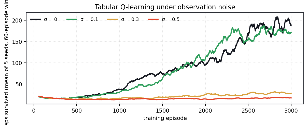
Everything below is the real experiment: Gymnasium's CartPole-v1 dynamics, the project's noise wrapper, and its tabular Q-learning, all running in your browser. Three thousand episodes take about a quarter of a second, so you can turn a knob and see the answer immediately instead of reading about it.
When the noise is above zero the dashed pole is what the agent sees; the solid one is where it actually is. Try balancing it yourself at σ = 0.3.
The original study compared Q-learning, DQN, PPO and SAC and concluded that PPO and SAC are the stable ones. Re-running the tabular half of it — five seeds, three thousand episodes each, everything in scripts/tools/run_clearnet.py — turned up three results that change how you would set the thing up.
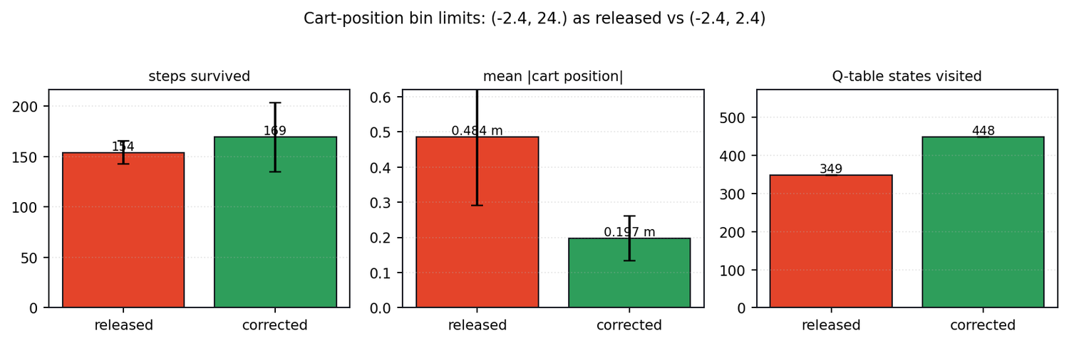
The released QLearning.py discretises cart position over (-2.4, 24.). Almost certainly a typo for (-2.4, 2.4) — and it matters, because reachable positions then occupy 18 % of that range, so with 8 bins every legal cart position falls in bin 0 or 1 and the other six are never visited.
The surprise is what it costs. Survival barely moves: 153.9 ± 11.3 steps as released against 169.1 ± 34.1 corrected, well inside the seed spread. But the mean distance of the cart from centre goes from 0.484 m to 0.197 m — cut by two and a half times. The poster reports that "the agent still suffered from drifting during testing" and attributes it to the reward function not asking the cart to stay centred. A good part of it is that the agent could not see where the cart was.
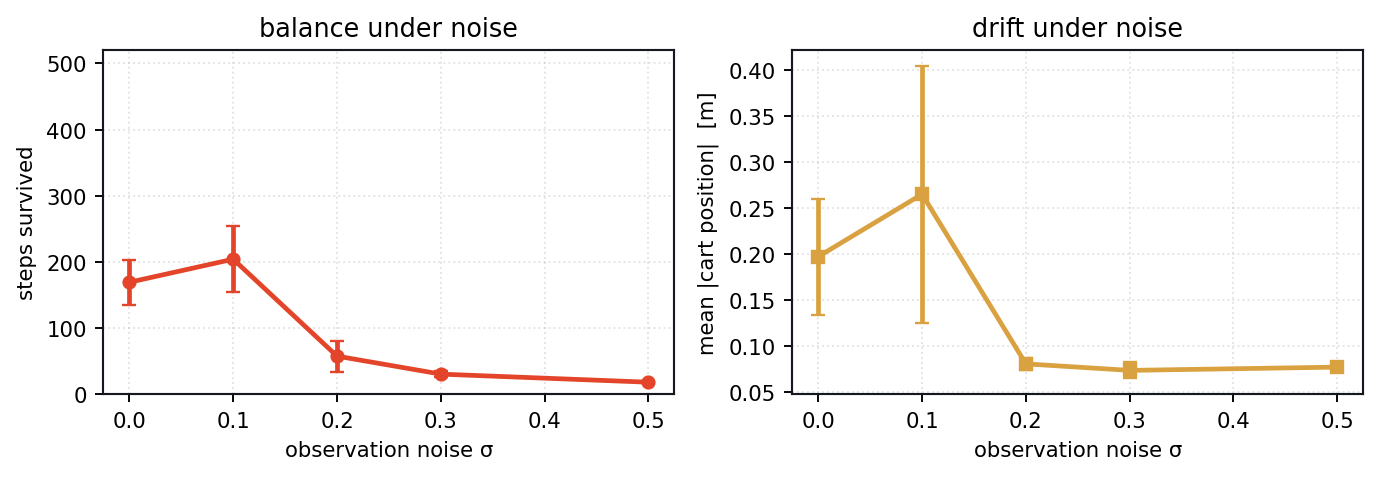
Survival peaks at σ = 0.1 — 203.9 ± 49.9 steps against 169.1 ± 34.1 with a perfectly clean observation — and then falls off a cliff: 57 steps at σ = 0.2, 30 at 0.3, 18 at 0.5. Mild observation noise behaves like exploration and like a smoothing prior over neighbouring bins, which is exactly what a sparse tabular value function wants. Past about σ = 0.15 the noise is larger than a bin and the discretisation stops meaning anything.
The poster's version of this is that "models trained with higher noise performed better under similar noise conditions but worse when the noise level was reduced". That is true, and there is also an optimum, and it is close to the bottom of the range they swept.
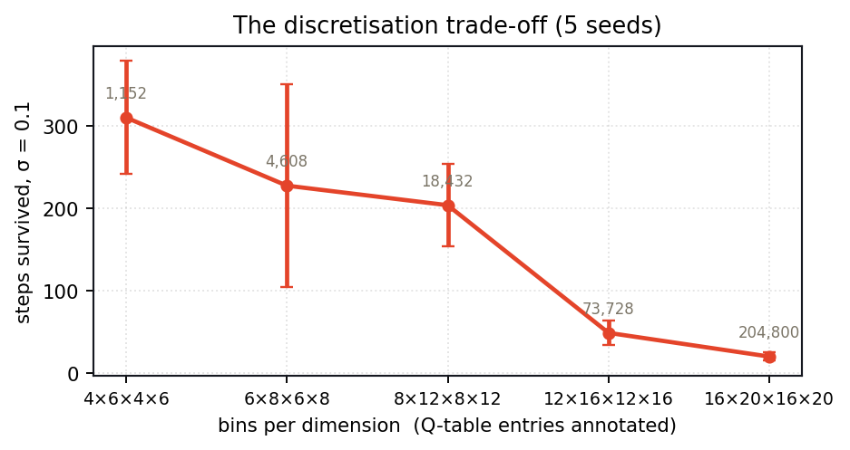
The poster picks 8×12×8×12 "for its fast convergence and stability". Sweeping the grid at a fixed budget of 3,000 episodes says something sharper: 4×6×4×6 survives 310 steps and 16×20×16×20 survives 20, a fifteen-fold difference, and the poster's choice sits in the middle at 204.
This is the curse of dimensionality doing exactly what it says on the tin. A 16×20×16×20 table has 204,800 entries; three thousand episodes of a few hundred steps is on the order of half a million transitions, so most entries are visited once or never. The finer grid is not worse in the limit — it is worse at this budget, and the budget is the thing you actually have.
Every method on this page is an answer to the same question, and they differ only in what they are willing to approximate. Setting the problem up properly makes the family tree obvious, so here is the whole derivation — from the Bellman equation to the entropy-regularised actor that ends up working best.
Cart-pole is a Markov decision process (𝒮, 𝒜, P, r, γ). The state is s = [x, ẋ, θ, θ̇], the action a ∈ {left, right} is a ±10 N impulse, and the reward is +1 for every step the pole stays up. The agent wants a policy π(a|s) maximising the expected discounted return:
Two value functions follow, and the Bellman equations that define them:
The second is the optimality equation, and it is a contraction: the Bellman operator 𝒯 satisfies ‖𝒯Q₁ − 𝒯Q₂‖∞ ≤ γ‖Q₁ − Q₂‖∞, so iterating it converges to the unique fixed point Q*. Everything below is a way of applying that operator without knowing P.
The wrinkle here is that the agent never sees s. It sees
which makes the process formally a POMDP. Every method below treats o as if it were s — a deliberate approximation, and the one the noise sweep is measuring the cost of.
Replace the expectation in the optimality equation with a single sample and take a step towards it. That is the whole algorithm:
The bracket is the temporal-difference error δt. Q-learning is off-policy: the max makes the target independent of the behaviour policy, so it can learn the greedy policy while exploring with an ε-greedy one,
and it converges to Q* with probability 1 provided every pair is visited infinitely often and the step sizes satisfy the Robbins–Monro conditions Σαt = ∞, Σαt² < ∞.
Neither condition survives contact with a continuous state. The table needs a finite index, so each dimension is binned:
with n = (8, 12, 8, 12), giving Π ni × |𝒜| = 18,432 entries. Two things break here, and both are measured above. The bins alias states that are genuinely different, which turns the MDP into a POMDP a second time over; and "visited infinitely often" becomes a budget question — at 3,000 episodes a 16×20×16×20 table sees most of its entries once or never, which is why the coarse grid wins. The choice of ℓi, ui is not innocent either, as finding 1 shows.
Drop the table for a function approximator Qφ(s,a) and fit it by regression onto the Bellman target:
Two details in that line are the entire reason DQN works at all.
The replay buffer 𝒟. Consecutive transitions in an episode are strongly correlated, and stochastic gradient descent assumes they are not. Sampling uniformly from a buffer of the last 10⁴ transitions decorrelates them and reuses each one many times, which matters when samples cost simulator time.
The target network φ⁻. Without it the regression target moves every time the parameters do, and the fixed point of the Bellman operator becomes a moving target chasing itself. Freezing a copy every C steps — or Polyak-averaging it — restores something closer to supervised regression. The price is bias: the target lags.
The max is also biased. Because 𝔼[max X] ≥ max 𝔼[X], taking a maximum over noisy estimates systematically overestimates. Double DQN splits the argmax from the evaluation and largely removes it:
What none of this fixes is catastrophic forgetting. The buffer is a sliding window, so as the policy improves the distribution in it shifts; the network fits the new region and quietly loses the old one, and the return curve falls off a cliff for no visible reason. It is the dominant failure mode of DQN on this problem, and it is why the next two methods constrain how far the policy may move in one update.
Hyperparameters used: γ = 0.9, α = 10⁻⁴ (Adam), batch 64, buffer 10⁴, ε: 0.99 → 0.01 with decay 0.9995.
Instead of learning values and reading a policy off them, parameterise the policy directly and differentiate the objective. The policy gradient theorem gives the gradient without differentiating the environment:
with the advantage Aπ(s,a) = Qπ(s,a) − Vπ(s). Subtracting V is what makes it usable: it is a baseline that leaves the gradient unbiased (because 𝔼a∼π[∇log π] = 0) while cutting the variance enormously. In practice A is estimated by generalised advantage estimation,
which interpolates between the low-variance, high-bias TD estimate (λ = 0) and the unbiased, high-variance Monte Carlo one (λ = 1).
The trouble with plain REINFORCE is that it is on-policy: every sample must come from the current πθ, so each batch is used once and a step that is slightly too large destroys the policy that generated it. Importance sampling lets a batch be reused,
but only while the ratio stays near 1; far from it the estimator's variance explodes. TRPO enforces that with a hard KL trust region, max ℒIS s.t. 𝔼[DKL(πθold‖πθ)] ≤ δ, which needs a constrained second-order solve. PPO gets the same effect with a first-order trick — clip the ratio and take the pessimistic branch:
Read the two cases. If  > 0 the objective stops improving once r exceeds 1+ϵ, so there is no gradient pulling the policy further towards an action it already prefers. If  < 0 it stops once r falls below 1−ϵ. Either way the update cannot move the policy far in one step, which is exactly the property DQN lacks — and it is why PPO's curve on this problem is the smooth one. Used here with ϵ = 0.2, γ = 0.99, 10 epochs per batch of 64.
SAC changes the objective rather than the optimiser. Add the policy's entropy to the reward, so the agent is paid to stay uncertain:
The Bellman equations pick up the entropy term and become soft:
and the optimal policy is no longer a delta function but a Boltzmann distribution over Q, π*(a|s) ∝ exp(Qsoft(s,a)/α). That is worth dwelling on: exploration is no longer bolted on as an ε that has to be scheduled down by hand, it falls out of the objective. It is the reason SAC converges fastest here — there is one fewer schedule to get wrong.
The critics are fitted to the soft target, with twin networks and a minimum to counter the same overestimation bias Double DQN addresses:
The actor minimises the KL divergence to that Boltzmann policy, which reduces to
and is differentiated through the reparameterisation a = fθ(s, ξ) = tanh(μθ(s) + σθ(s) ⊙ ξ), ξ ∼ 𝒩(0, I), which gives a pathwise gradient with far lower variance than the score-function estimator a policy gradient would use. The tanh squashing needs its Jacobian in the log-likelihood: log π(a|s) = log 𝒩(u|μ,σ) − Σi log(1 − tanh²(ui)). And α itself can be learned, by treating the entropy as a constraint with target ℋ̄:
One catch: all of that assumes a continuous action space, and cart-pole's is binary. The project bridges it with an action-space wrapper — SAC produces a scalar in [−1, 1] which is thresholded into left/right. That works, but it is worth being honest that it is a workaround; the principled version is discrete SAC, which takes the expectation over actions analytically instead of sampling. Used here with γ = 0.99, τ = 0.005, α = 0.2, lr = 3×10⁻⁴, batch 64, buffer 10⁵.
The environment's reward is +1 per step, which says nothing about where the cart should be. The project replaces it with a shaped version that asks for the middle of the track and an upright pole, and penalises ending early:
Shaping is not free. Ng, Harada and Russell showed that the only class of shaping guaranteed to leave the optimal policy unchanged is potential-based, F(s,a,s′) = γΦ(s′) − Φ(s), for any Φ. The shaping above is not of that form — it is a state-dependent bonus, so it changes the optimal policy, which here is the intent: a controller that balances the pole while wandering to the end of the track is not the controller anyone wanted.
The finding worth carrying away is that shaping was not the whole story. The poster attributes the residual drift to the reward not asking for a centred cart. Finding 1 shows a good part of it was that the agent could not see where the cart was, because the discretisation had collapsed cart position into two bins. Shaping the reward is the natural first thing to reach for, and it was treating a symptom.
The environment is Gymnasium's CartPole-v1: a cart on a rail with an inverted pendulum on it, one binary action — push left or push right with a constant 10 N — and a reward of +1 for every step the pole stays up. The episode ends when the pole passes 12° or the cart passes 2.4 m, or at 500 steps.
What makes it a study rather than a tutorial is the observation wrapper. Every component of the state is corrupted before the agent sees it:
so σ scales a per-component range rather than being an absolute standard deviation — σ = 0.5 puts about a metre of noise on the cart position, which is nearly half the track.
Four controllers were compared. Tabular Q-learning quantises the four continuous states into bins and keeps one value per bin-action pair. DQN replaces the table with a network plus a target copy and a replay buffer, and converges far faster but suffers catastrophic forgetting. PPO keeps its updates inside a trust region and is the most stable over long training. SAC converges fastest of all — the entropy term removes the ε-decay schedule entirely — and needs an action-space wrapper to work on this discrete problem at all.
The reward was reshaped from the plain +1: reward the cart for staying near the middle and the pole for staying upright, and penalise heavily if the episode ends before 500 steps. That is the change the poster credits for fixing the drift — see finding 1 for the part it does not.
The original demo reel: Q-learning holding up under σ = 0.1, then the same controller as the training noise is raised, then the deep methods.
| Method | Converges | Stability |
|---|---|---|
| Tabular Q-learning | slowest | curse of dimensionality |
| DQN | fast | catastrophic forgetting |
| PPO | medium | most stable |
| SAC | fastest | stable |
The sandbox above runs assets/js/clearnet_cartpole.js, the same dynamics, noise model and Q-learning update as scripts/tools/cartpole.py. Single runs are noisy — the numbers quoted in the findings are five-seed means, and the sandbox trains one seed at a time, so expect to see the spread.
ECE 1508: Reinforcement Learning (Summer 2024) at the University of Toronto, joint work with Aravind Narayanan — equal contribution. The environment is Gymnasium's CartPole-v1.
The four controllers, the noise wrapper and the demo reel are from the course project. The five-seed re-run, the three findings above and the browser sandbox were built afterwards, on the released code.