Certifiably Correct Hand-Eye Calibration

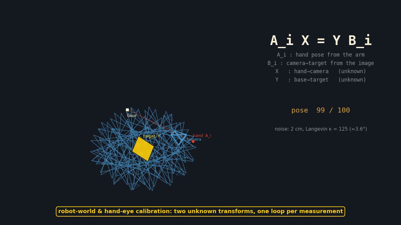
Fifteen seconds: a camera on a robot hand orbits a target, twenty-four local solves from random starts scatter into local minima, and the convex relaxation lands on the one certified answer. The full demo adds the simulation tables and the real rig.

Technical report Paper (arXiv) Original code (Julia)

−1.1e-8

duality gap, real rig

217-dimensional SDP, 24 poses at once; paper: −6.4e-9

2.5%

tag scale found

α = 1.0255 on the tag-derived translations: the paper's hand-measured tags were 2.5 % off

1–40%

local minima, random start

same objective, same data, local solver; the SDP never needs a start

2e-8

worst duality gap

over 1,600 simulated solves at four noise levels: the relaxation stayed tight every time

3.6mm

hand–camera error

poses on a sphere, κ = 125, σ = 1 cm, mean over 100 runs; linear two-stage: 7.5 mm

230s

real problem solved

16 tags × 8 cameras, 3,230 measurements, SCS on a laptop; unknown scale in 81 s

The problem, in fifteen seconds

What is measured

A_i: the pose of the hand (or of the rig, from motion capture) at every time i.
B_i: the pose of a fiducial target as the camera sees it, from an AprilTag detector with a hand-measured tag size.
Which camera saw which tag: a bipartite graph. On the real rig, 16 tags, 8 cameras, 73 edges, 3,230 pose pairs.

What we want

X_j: where each tag sits in the world.
Y_k: where each camera sits on the hand. That is the calibration.
α: the true tag scale, when the hand-measured size cannot be trusted (the monocular case).

The insight

Every observation closes a loop: A_iX_j = Y_kB_i.
The rotations make the least-squares fit non-convex, so a local solver can stop in the wrong valley without warning.
Lift the rotations into a positive-semidefinite matrix, drop the rank-one condition, and the relaxed problem is convex: no initial guess, and a duality gap that proves the answer is the global optimum.

In one strip

A camera orbiting an AprilTag target with the base, hand and target frames

1 · Loop

A_i X = Y B_i

The arm reports the hand pose A_i; the camera reports the target pose B_i. The unknowns are hand→camera X and base→target Y. With several cameras and several targets it is a bipartite graph of such loops, and a monocular camera adds an unknown scale α.

Twenty-four local solves scattering into local minima next to the certified SDP optimum

2 · Relax

Rotations only, then lift

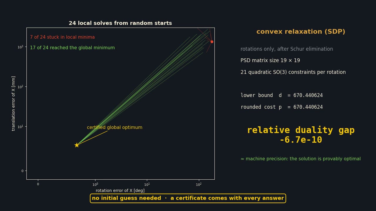
Translations and α are eliminated by a Schur complement. Each rotation becomes nine numbers with 21 quadratic constraints; the Shor relaxation is a semidefinite program whose value bounds the true cost from below. If the rounded answer meets the bound, it is provably optimal.

Eight camera poses recovered from the real rig and the residual distribution

3 · Certify

Eight cameras, sixteen tags, one problem

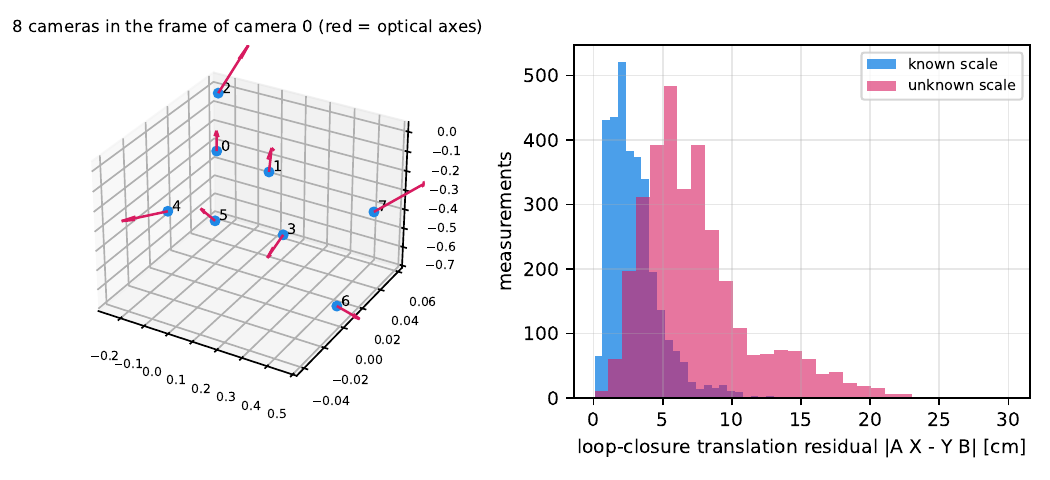
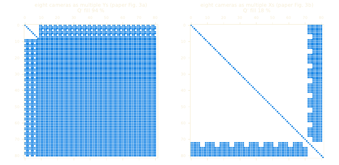
The published rig data: 73 camera–tag pairs, 3,230 pose pairs. One 217-dimensional SDP returns all 24 poses with a duality gap at machine precision, and with the scale free it reports the tags 2.5 % smaller than measured, as the paper found.

Try it live

LIVE DEMO · runs in your browser

Mount the camera, place the target, orbit, certify

Set the unknown transforms yourself: X (hand → camera) and Y (base → target), the rotation noise concentration κ and the translation noise σ of the camera's target measurements, and how many poses the arm visits. Press Orbit & calibrate: the camera orbits the target on a sphere, every pose closes one loop A_iX = YB_i, and three solvers run live on the same objective: the linear two-stage closed form, a local Levenberg–Marquardt solver from eight random starts, and the paper's semidefinite relaxation (translations Schur-eliminated, both rotations lifted into a 19×19 matrix with the 42 quadratic SO(3) constraints) solved by an ADMM iteration with the rank check and the duality-gap certificate. Drag the 3-D view to orbit.

X roll X pitch X yaw X offset Y yaw Y offset x

rotation noise κ translation noise σ poses on the sphere

no run yet

solver log will appear here

Method

The maximum-likelihood cost is a sum over every loop of a translation term and a chordal rotation term, both quadratic in the unknowns once the rotation matrices are vectorised:

J = ½ Σ ( 1/σ² ‖ RA tX + α tA − tY − RY tB ‖² + κ ‖ RA RX − RY RB ‖F² )

The translations and the scale appear without constraints, so they are solved out by a generalized Schur complement, leaving a quadratic form in the rotations alone. Each rotation is kept in SO(3) by 21 homogenised quadratic constraints (row and column orthonormality plus the right-hand rule), and the relaxation drops the rank-one condition on the lifted variable.

Noise model (paper §8): translations get Gaussian noise N(0, σ²I); rotations get isotropic Langevin noise, p(R) ∝ exp(κ tr(R̄ᵀR)), sampled by rejection. κ = 125 is about 3.6° of angular error, κ = 12 about 12°.
Identifiability (Theorem 3, Corollary 4): on a weakly connected graph, one sensor–target edge with three measurements whose relative rotations have distinct principal axes fixes that edge, and every other X and Y follows by propagating loop closures across the graph. The re-run checks this criterion on each edge of the real data.
Tightness (Proposition 7): for noise-free data with a unique solution the relaxation is exact, and it stays tight under moderate noise. The certificate is ρ̂ = (p − d)/|d| between the rounded cost and the SDP bound, plus the eigenvalue ratio λ₂/λ₁ of the lifted matrix.
Solver: the primal SDP in cvxpy, SCS at 10⁻¹¹ with a Clarabel fallback; leading-eigenvector rounding, per-block SO(3) projection, translations and α back-substituted.
Baselines: a linear two-stage solver in the Shah / Wang style and a local Levenberg–Marquardt solver on the same objective, started at random, from the linear solution, or (unknown scale) 10° and 10 cm from the truth.

cvxpy + SCS / ClarabelLangevin sampling by rejectionsharded campaignspaper's real CSVs

Grid of which camera saw which tag, coloured by identifiability — **The measurement graph** (paper Fig. 10): blue pairs satisfy the two-axis criterion on their own, red pairs were seen but need the rest of the graph, numbers are pose pairs. 52 of 73 edges are identifiable alone; the graph is connected, so the whole problem is.

Sparsity pattern of the quadratic-form matrices before and after Schur elimination — **Sparsity after the Schur complement** (the paper’s Figs. 3–4): the same eight-camera rig modelled as one shared X with eight Ys (left) fills the reduced matrix Q′ almost completely, while modelled as eight Xs with one Y (right) it leaves a block-diagonal-plus-border pattern the solver can exploit. Which side of the loop the unknowns sit on changes the cost of the SDP.

Simulation studies

Setup

The setup: what is given, what is estimated

A camera on a robot hand visits poses on a sphere around a fiducial target; the ledger of knowns, unknowns and ground truth appears alongside the measurements as they are taken.

Recording

The campaign, recorded

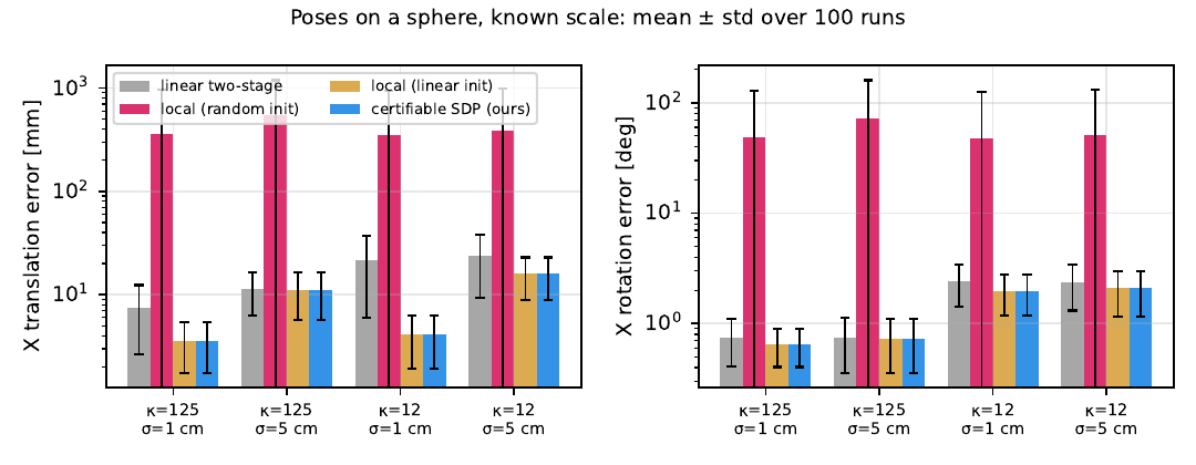
Four noise levels, one hundred seeded runs each, four solvers per run. Every random-start local solve lands on the error axis as it finishes; the certified SDP points stack at the bottom.

Given

Hand poses A_i with translation noise σ ∈ {{1, 5}} cm and Langevin rotation noise κ ∈ {{125, 12}}.
Target poses B_i with the same noise; in the monocular study their translations are scaled by α = 0.5.
Sphere study: 100 poses on a sphere around one target. Four-camera study: 108 poses, four fixed cameras watching a target on the hand.

Estimated

X (hand–camera, or the target on the hand) and Y (world–base, or each of the four cameras).
α in the monocular study.
Four solvers on identical data: linear two-stage, local LM from random starts, local LM from the linear solution, and the certified SDP.

Ground truth and protocol

Random rigid transforms per run, fixed seeds, 100 runs per noise level: 1,600 SDP solves plus baselines.
Errors: translation of X and Y in mm, chordal rotation error in degrees, scale error in percent.
The certificate is recorded for every solve: relative gap, eigenvalue ratio, solver time.

End-effector rotation and translation over the 100 sphere poses — **The pose sequence of the sphere study** (from the thesis figures): end-effector rotation and translation against pose number. The rotations sweep about several axes, which is what Corollary 4 asks for.

End-effector rotation and translation over the 108 four-camera poses — **The four-camera sequence**: 108 poses that keep the hand-mounted target in every camera’s view in turn.

Poses on a sphere, known scale (paper Table 2)

Bar chart of hand–camera errors per method and noise level, poses on a sphere — **Re-run.** The certified SDP and the well-started local solver agree to a tenth of a millimetre (same objective, tight relaxation), both beat the linear two-stage method, and the local solver from random starts is off by hundreds of millimetres in 26–40 % of runs.

Maximum duality gap per study and noise level — **The certificate never failed.** Largest relative duality gap over all 1,600 solves: 2e-8; largest λ₂/λ₁: 3e-11. Tight at κ = 12, σ = 5 cm too, beyond what Proposition 7 promises.

noise	method	t_X err [mm]	r_X err [deg]	t_Y err [mm]	r_Y err [deg]
κ=125, σ=1 cm	linear two-stage	7.50 ± 4.88	0.75 ± 0.34	1.92 ± 0.93	0.75 ± 0.34
	local (random init)	362.69 ± 590.64	48.98 ± 79.49	2.06 ± 1.07	48.74 ± 79.79
	local (linear init)	3.58 ± 1.83	0.65 ± 0.24	1.93 ± 0.94	0.22 ± 0.13
	SDP (ours)	3.58 ± 1.83	0.65 ± 0.24	1.93 ± 0.94	0.22 ± 0.13
κ=125, σ=5 cm	linear two-stage	11.28 ± 5.07	0.74 ± 0.39	9.03 ± 4.24	0.74 ± 0.29
	local (random init)	540.23 ± 648.30	72.26 ± 87.57	9.02 ± 4.33	72.23 ± 87.74
	local (linear init)	10.95 ± 5.31	0.73 ± 0.37	9.03 ± 4.24	0.59 ± 0.32
	SDP (ours)	10.95 ± 5.31	0.73 ± 0.37	9.03 ± 4.24	0.59 ± 0.32
κ=12, σ=1 cm	linear two-stage	21.70 ± 15.74	2.42 ± 0.99	2.05 ± 0.95	2.26 ± 1.04
	local (random init)	350.07 ± 583.44	47.89 ± 77.53	2.50 ± 1.65	46.97 ± 78.77
	local (linear init)	4.09 ± 2.17	1.97 ± 0.80	2.05 ± 0.93	0.26 ± 0.16
	SDP (ours)	4.09 ± 2.17	1.97 ± 0.80	2.05 ± 0.93	0.26 ± 0.16
κ=12, σ=5 cm	linear two-stage	23.62 ± 14.32	2.36 ± 1.04	9.04 ± 4.16	2.27 ± 1.03
	local (random init)	385.60 ± 594.33	51.38 ± 79.29	9.11 ± 4.13	50.97 ± 80.23
	local (linear init)	15.85 ± 7.07	2.08 ± 0.93	9.05 ± 4.14	0.95 ± 0.49
	SDP (ours)	15.85 ± 7.07	2.08 ± 0.93	9.05 ± 4.14	0.95 ± 0.49

← scroll the table sideways →

Mean ± std over 100 runs. Absolute values differ from the paper’s table because its sphere geometry and random transforms are not specified; the ordering of the methods is what is reproduced.

Four fixed cameras, known scale (paper Table 4)

Four fixed cameras observing a hand-mounted target: errors per method — **Five rotations solved jointly** in one 46×46 SDP. Camera rotations to 0.31° (linear: 0.58°) and camera translations to 7.9 mm (linear: 14.4 mm) at the lowest noise; t_Y and r_Y are averaged over the four cameras.

Why the local solver fails less here.

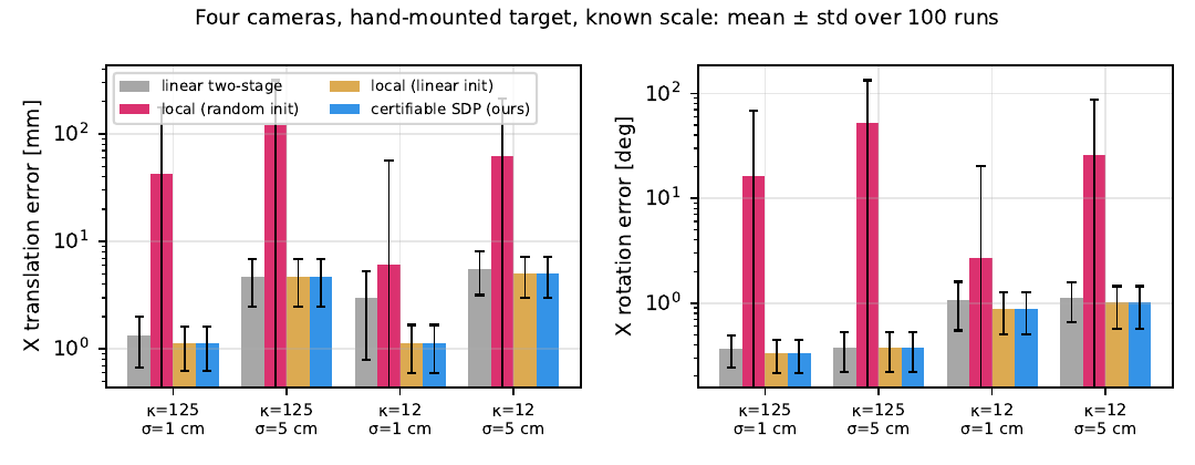
With four cameras every hand pose closes four loops, and the random-start local solver finds a wrong minimum in only 1–29 % of runs against 26–40 % on the sphere. It still fails. The SDP solves the 46-dimensional lifted problem in 5–16 s and certifies every one of the 400 runs.

noise	method	t_X err [mm]	r_X err [deg]	t_Y err [mm]	r_Y err [deg]
κ=125, σ=1 cm	linear two-stage	1.34 ± 0.67	0.36 ± 0.12	14.36 ± 4.17	0.58 ± 0.13
	local (random init)	42.40 ± 132.96	16.48 ± 51.37	234.72 ± 725.11	16.42 ± 51.22
	local (linear init)	1.13 ± 0.50	0.33 ± 0.11	7.87 ± 2.67	0.31 ± 0.09
	SDP (ours)	1.13 ± 0.50	0.33 ± 0.11	7.87 ± 2.67	0.31 ± 0.09
κ=125, σ=5 cm	linear two-stage	4.70 ± 2.21	0.37 ± 0.15	17.00 ± 4.43	0.60 ± 0.14
	local (random init)	119.99 ± 196.30	52.40 ± 81.41	775.58 ± 1193.33	52.49 ± 81.26
	local (linear init)	4.67 ± 2.22	0.37 ± 0.15	16.24 ± 4.35	0.56 ± 0.13
	SDP (ours)	4.67 ± 2.22	0.37 ± 0.15	16.24 ± 4.35	0.56 ± 0.13
κ=12, σ=1 cm	linear two-stage	3.02 ± 2.23	1.07 ± 0.52	48.59 ± 13.96	1.92 ± 0.44
	local (random init)	6.16 ± 50.13	2.67 ± 17.82	37.96 ± 281.75	2.18 ± 17.85
	local (linear init)	1.13 ± 0.54	0.88 ± 0.37	9.63 ± 3.68	0.38 ± 0.13
	SDP (ours)	1.13 ± 0.54	0.88 ± 0.37	9.63 ± 3.68	0.38 ± 0.13
κ=12, σ=5 cm	linear two-stage	5.61 ± 2.43	1.11 ± 0.46	47.16 ± 13.70	1.99 ± 0.45
	local (random init)	62.69 ± 152.15	25.97 ± 61.85	398.15 ± 912.46	26.11 ± 61.44
	local (linear init)	5.08 ± 2.06	1.01 ± 0.44	32.22 ± 10.13	1.33 ± 0.36
	SDP (ours)	5.08 ± 2.06	1.01 ± 0.44	32.22 ± 10.13	1.33 ± 0.36

← scroll the table sideways →

Unknown scale: the monocular case (paper Tables 3 and 5)

Unknown-scale sphere study: errors per method — **Two spheres, α = 0.5.** The scale comes back to 0.44 % at σ = 1 cm and 2.2 % at σ = 5 cm. The SDP needs no initial guess; the local solver is started 10° and 10 cm from the truth, and from random starts it diverges when α is free.

Unknown-scale four-camera study: errors per method — **Four cameras, α = 0.5.** Same picture: 0.6 % scale error at low noise, 2.9–3.1 % at σ = 5 cm, identical to the close-start local solution because the relaxation is tight.

noise	method	t_X err [mm]	r_X err [deg]	t_Y err [mm]	r_Y err [deg]	α_err [%]
κ=125, σ=1 cm	local (close init)	5.99 ± 2.71	0.64 ± 0.26	3.96 ± 1.70	0.35 ± 0.16	4.4e-1 ± 3.8e-1
	SDP (ours)	5.99 ± 2.71	0.64 ± 0.26	3.96 ± 1.70	0.35 ± 0.16	4.4e-1 ± 3.8e-1
κ=125, σ=5 cm	local (close init)	26.33 ± 11.86	0.68 ± 0.27	19.62 ± 8.43	0.67 ± 0.28	2.2 ± 1.6
	SDP (ours)	26.33 ± 11.86	0.68 ± 0.27	19.62 ± 8.43	0.67 ± 0.28	2.2 ± 1.6
κ=12, σ=1 cm	local (close init)	5.54 ± 2.56	1.83 ± 0.75	3.75 ± 1.63	0.37 ± 0.17	5.1e-1 ± 3.7e-1
	SDP (ours)	5.54 ± 2.56	1.83 ± 0.75	3.75 ± 1.63	0.37 ± 0.17	5.1e-1 ± 3.7e-1
κ=12, σ=5 cm	local (close init)	29.42 ± 12.46	2.10 ± 0.96	19.43 ± 7.99	1.58 ± 0.77	2.6 ± 1.6
	SDP (ours)	29.42 ± 12.46	2.10 ± 0.96	19.43 ± 7.99	1.58 ± 0.77	2.6 ± 1.6

← scroll the table sideways →

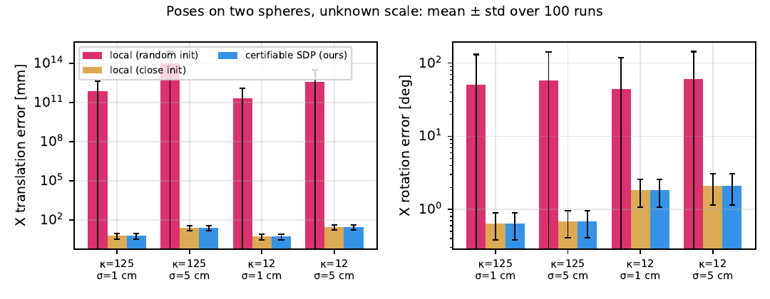
Sphere study, unknown scale.

noise	method	t_X err [mm]	r_X err [deg]	t_Y err [mm]	r_Y err [deg]	α_err [%]
κ=125, σ=1 cm	local (close init)	2.99 ± 1.68	0.31 ± 0.15	17.17 ± 6.21	0.45 ± 0.11	6.1e-1 ± 4.5e-1
	SDP (ours)	2.99 ± 1.68	0.31 ± 0.15	17.17 ± 6.21	0.45 ± 0.11	6.1e-1 ± 4.5e-1
κ=125, σ=5 cm	local (close init)	14.57 ± 8.52	0.35 ± 0.16	57.41 ± 33.30	0.59 ± 0.12	2.9 ± 2.1
	SDP (ours)	14.57 ± 8.52	0.35 ± 0.16	57.41 ± 33.30	0.59 ± 0.12	2.9 ± 2.1
κ=12, σ=1 cm	local (close init)	3.18 ± 1.40	0.92 ± 0.38	21.86 ± 7.97	0.69 ± 0.24	5.9e-1 ± 4.4e-1
	SDP (ours)	3.18 ± 1.40	0.92 ± 0.38	21.86 ± 7.97	0.69 ± 0.24	5.9e-1 ± 4.4e-1
κ=12, σ=5 cm	local (close init)	15.05 ± 7.26	1.01 ± 0.46	75.29 ± 31.46	1.73 ± 0.38	3.1 ± 2.4
	SDP (ours)	15.05 ± 7.26	1.01 ± 0.46	75.29 ± 31.46	1.73 ± 0.38	3.1 ± 2.4

← scroll the table sideways →

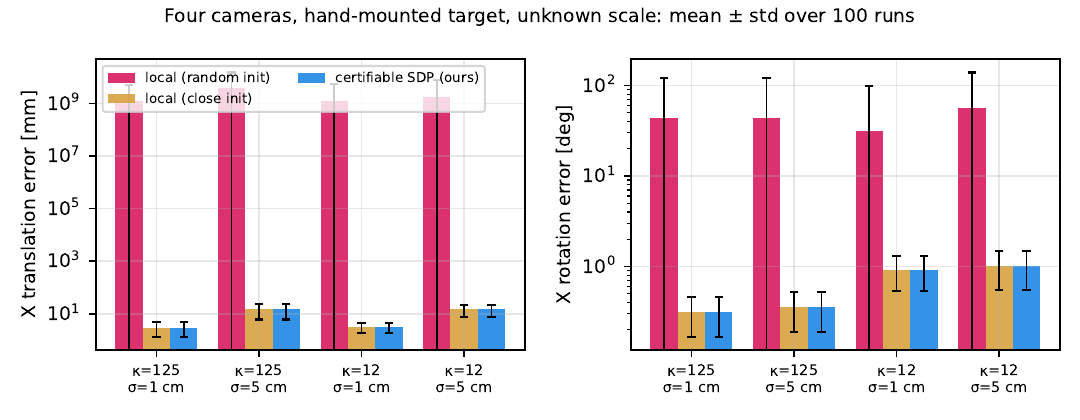
Four-camera study, unknown scale.

Certificate and runtime, every setting

study	κ	σ [cm]	median ρ̂	max \|ρ̂\|	max λ₂/λ₁	local minima (random init)	SDP time [s]
sphere, known scale	125	1	-8.9e-10	1.7e-8	3.8e-12	27%	0.39
sphere, known scale	125	5	-3.1e-9	1.2e-8	2.2e-11	40%	3.44
sphere, known scale	12	1	+1.1e-12	1.9e-8	6.0e-12	26%	0.26
sphere, known scale	12	5	+9.3e-11	4.1e-10	4.0e-12	28%	0.24
sphere, unknown scale	125	1	-6.2e-10	5.0e-9	8.7e-12	28%	2.36
sphere, unknown scale	125	5	-4.4e-9	1.9e-8	3.4e-11	33%	3.51
sphere, unknown scale	12	1	-5.1e-13	2.6e-9	4.2e-12	24%	0.25
sphere, unknown scale	12	5	-2.0e-10	9.0e-10	1.9e-11	33%	3.44
4 cameras, known scale	125	1	+1.3e-9	7.5e-9	1.0e-11	9%	16.00
4 cameras, known scale	125	5	+1.4e-9	5.2e-9	6.7e-12	29%	11.97
4 cameras, known scale	12	1	+1.3e-10	7.4e-9	9.6e-12	1%	4.82
4 cameras, known scale	12	5	+1.2e-10	5.7e-10	8.5e-12	14%	8.36
4 cameras, unknown scale	125	1	+9.7e-10	6.0e-9	8.3e-12	24%	8.32
4 cameras, unknown scale	125	5	+1.0e-9	4.9e-9	6.3e-12	25%	6.85
4 cameras, unknown scale	12	1	+1.0e-10	3.4e-9	8.8e-12	17%	4.56
4 cameras, unknown scale	12	5	+1.3e-10	5.4e-10	7.5e-12	31%	5.69

← scroll the table sideways →

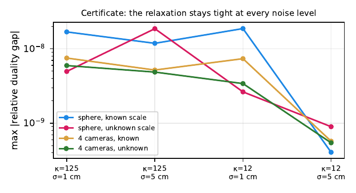
Median and worst relative duality gap, worst eigenvalue ratio, fraction of random-start local solves that ended in a local minimum, and SCS solve time on a laptop. The paper reports at most seven seconds per synthetic problem with COSMO; the real problem below takes 230 s here.

The real rig

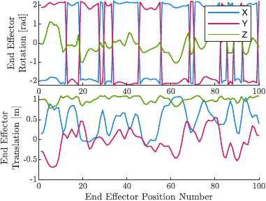
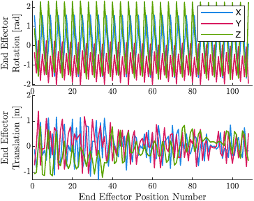
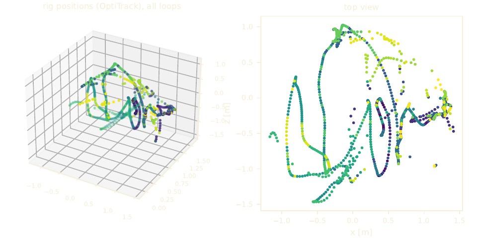
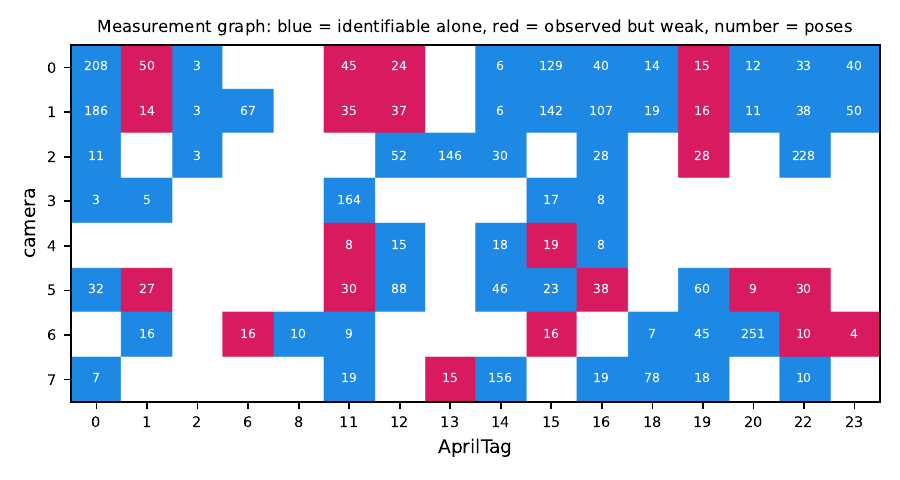
The paper’s experiment from its public data: the OptiTrack trajectory of the eight-camera rig through a motion-capture room, the sixteen AprilTags, which camera sees which tag as the rig moves, the measurement graph filling in, and the certified camera cluster.

INTERACTIVE 3-D · REAL DATA

The experiment, rebuilt from the published measurements

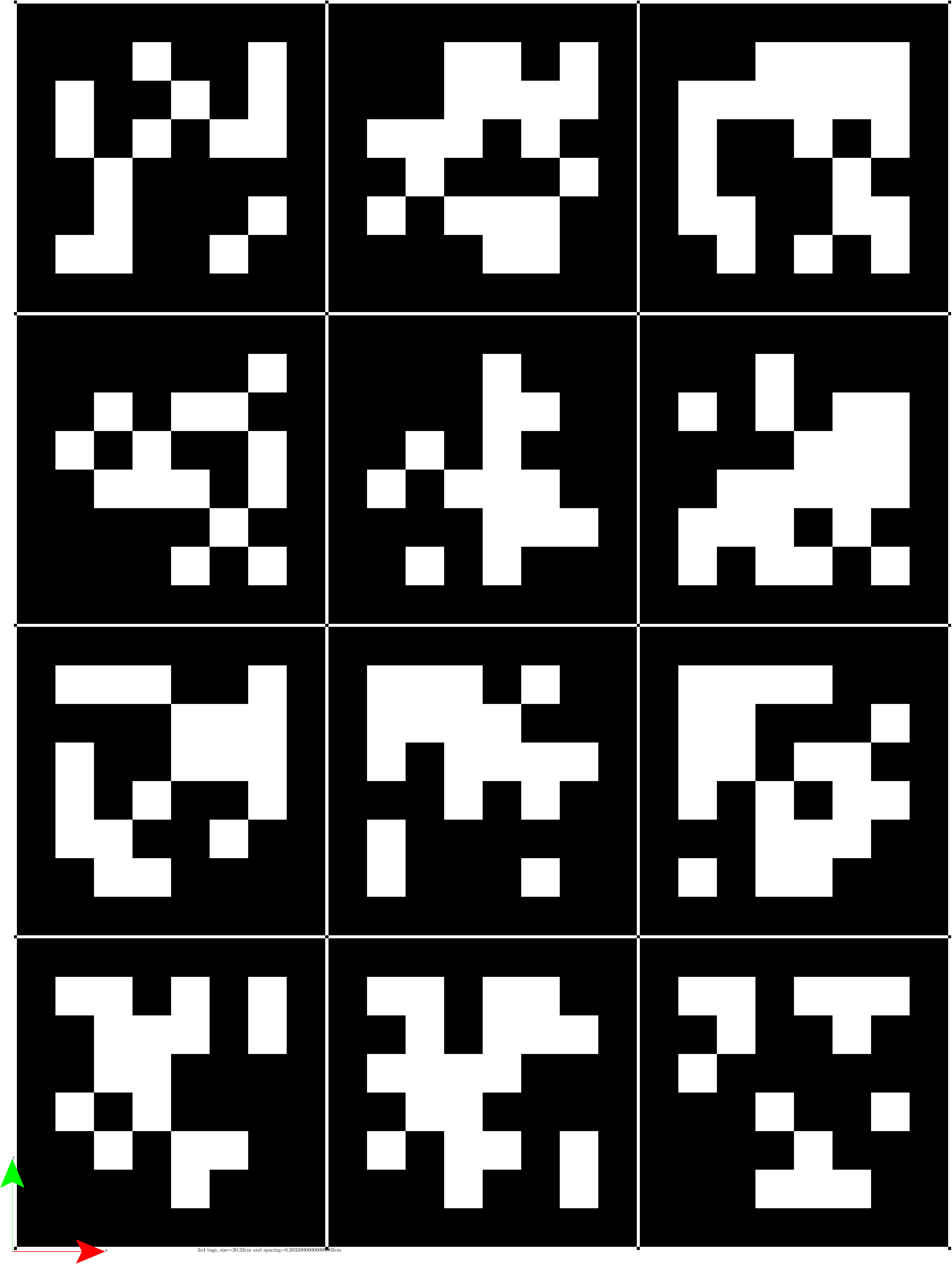
The OptiTrack world of the paper’s motion-capture room: the sixteen AprilTags at their certified poses (true 20.3 cm size, real tag36h11 patterns), the eight-camera rig replayed along its trajectory at constant walking speed, cameras lighting up when they detect a tag, and the loop A_iX_j = Y_kB_i drawn as a ray for every detection. Drag to orbit, right-drag to pan, wheel to zoom, click any tag or camera.

speed pose 1 / 1083 follow the rig trajectory detections frustums labels

Loading the scene…

INTERACTIVE 3-D · RESULTS

The certified answer, in three dimensions

Rotate the eight-camera cluster the SDP certified, compare it with where the linear two-stage method put each camera, and switch to the tag constellation to see which tags the loop closures pin down well and which the linear solution had wrong by tens of centimetres.

view linear two-stage correction arrows unknown-scale solution

Loading…

Who saw what, and when

Each row is a camera, the horizontal axis is the rig’s path (1,083 poses), every tick is one detection coloured by tag. Long runs are a camera holding a tag in view; the gaps are the rig turning away.

Every loop closure’s residual along the path

|A_iX_j − Y_kB_i| in cm for all 3,230 measurements at the certified solution, coloured by camera, with the median. No camera and no stretch of the path is systematically worse: the rest is detection noise.

Excitation map of one camera–tag edge

edge

Corollary 4 made visible: each dot is the axis of the rig’s rotation between the first and a later observation of this pair (azimuth, elevation), sized by the angle. Two clearly distinct axes and the edge identifies both transforms on its own; dots on one line mean the edge needs the rest of the graph.

Detections per tag, and by whom

Stacked by camera. Tags 0, 1 and 2 near the start of the path dominate; a few tags were seen by only one or two cameras, which is exactly where the bipartite graph, not a single edge, carries the identifiability.

The certificate as a picture: the spectrum of the lifted matrix

All 217 eigenvalues of the SDP solution Z. A tight relaxation has exactly one non-zero eigenvalue: the rest sit at solver precision, twelve orders of magnitude below, which is what lets the rank-one factor be read off as the certified rotations.

Motion-capture room with AprilTags on a dark wall

Second view of the room with AprilTags on stands and boxes

The data-collection rig with eight cameras and OptiTrack markers

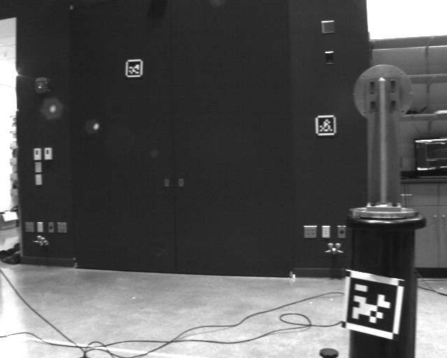
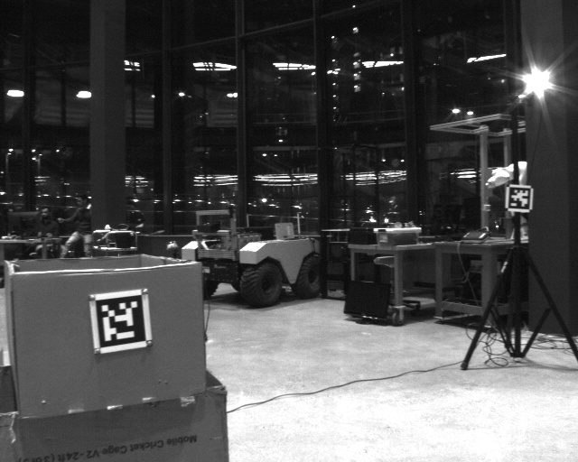
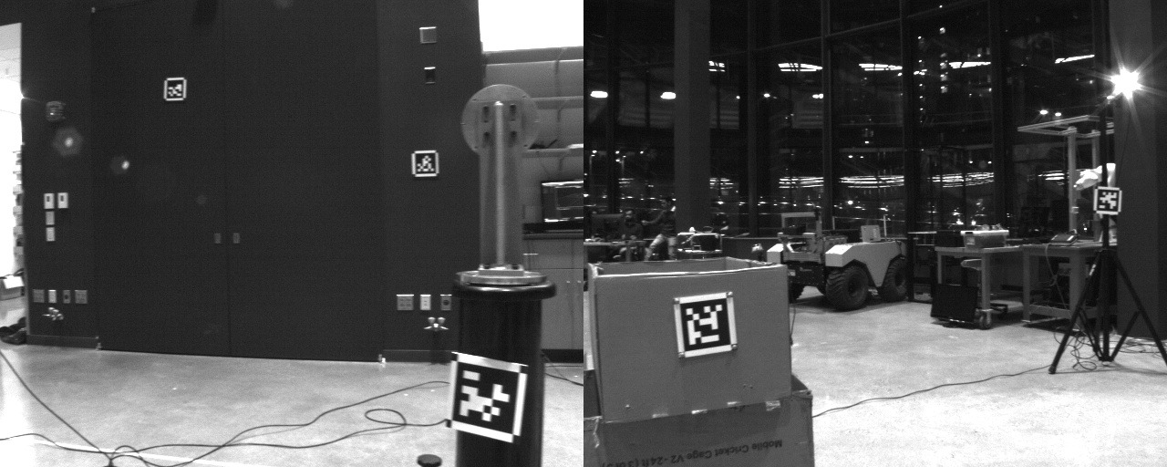
Paper Figs. 7–8: the environment seen from camera 0, and the rig. Eight hardware-synchronised Point Grey Blackfly S cameras, OptiTrack markers and a VectorNav VN-100. The tag at the bottom left of the middle image carries its own markers, so its world pose is ground truth.

Pipeline, as in the paper’s §9.1: OptiTrack gives the rig pose A, an AprilTag detector gives each camera-to-tag pose B, the two clocks are joined by interpolating OptiTrack onto the image timestamps, and a RANSAC on the loop closure X_j = A⁻¹Y_kB (inliers within 0.6 m and 60°) rejects bad detections before the batch solve.

The public repository ships the processed measurements. With the paper’s weights (κ = 125, σ = 0.1 m) the joint problem has 24 rotations, a 217×217 lifted matrix and 504 constraints. SCS solves it in 230 s with the scale known and 81 s with the scale free.

solve	duality gap ρ̂	λ₂/λ₁	α	median loop residual	paper
known scale	−1.09e-8	7.7e-13	1	2.5 cm / 1.3°	−6.41e-9
unknown scale	−1.19e-8	4.1e-12	1.0255	6.6 cm / 1.3°	8.55e-9, tags 2.5 % small

The certified solution coincides with the local solver started from the linear solution (cost 985.244 both), while the linear two-stage answer sits at 1027.3 and differs by up to 3.8 cm and 1.1° per camera. The paper found the same 2.5 % tag-scale error and traced it to a 3 mm mistake in the hand-measured tag size.

The rig trajectory from the public data, 3-D and top view coloured by time — **The rig’s trajectory** reconstructed from the public CSVs (the A poses), coloured by time; the paper’s own plot of it is its Fig. 9.

A sheet of AprilTags — **The tags** (tag36h11 family, paper Fig. 8): sixteen of them, on walls, stands and boxes, so that every camera sees several from most rig poses.

What the paper measured against Kalibr (its Table 6)

method (initialisation)	camera translation error [cm]	camera rotation error [°]	tag-20 translation error [cm]	tag-20 rotation error [°]
Wang et al. 2022 (linear)	3.46 ± 1.69	1.38 ± 0.81	11.7	5.30
local optimiser (Wang)	3.34 ± 2.44	0.88 ± 0.49	11.4	4.50
certified SDP	3.20 ± 1.88	0.99 ± 0.52	11.5	4.73
local optimiser, unknown scale (Wang)	3.28 ± 2.42	0.86 ± 0.47	7.92	4.50
certified SDP, unknown scale	2.87 ± 1.94	0.99 ± 0.52	7.94	4.72

← scroll the table sideways →

These are the paper’s numbers: the Kalibr camera extrinsics and the OptiTrack-marked tag it compares against are not in the public repository, so the re-run reports internal consistency instead (below). Freeing the scale cuts the tag-20 translation error from 11.5 to 7.9 cm.

The eight camera frames and the loop-closure residual histogram — **The certified camera cluster** (optical axes in red) and the distribution of loop-closure translation residuals |AX − YB| over the 3,230 measurements, known scale in blue and unknown scale in pink.

camera	baseline to cam 0 [cm]	roll [°]	pitch [°]	yaw [°]	unknown-scale baseline [cm]
cam 0	0.0	0.0	0.0	0.0	0.0
cam 1	22.2	-2.1	-2.8	-0.9	21.5
cam 2	25.0	-29.2	-56.9	0.4	25.6
cam 3	43.9	17.1	47.0	-1.6	44.4
cam 4	41.3	44.0	-81.8	-32.0	42.4
cam 5	64.1	118.3	-83.8	-122.8	65.2
cam 6	80.6	173.8	78.4	172.7	81.2
cam 7	57.6	-120.0	79.3	-87.0	59.0

← scroll the table sideways →

Certified known-scale solution in the frame of camera 0. The eight baselines (22–81 cm) agree between the known- and unknown-scale solutions to within 1.5 cm, the α = 1.0255 stretch.

What the re-run found

The paper's claims held; the notes below are about getting there from scratch.

1

The certificate is only as good as the solver's tolerance

An interior-point solver at 10⁻¹⁰ returned duality gaps of −1.5e-6: the rounded cost was below the bound, which cannot happen exactly and simply meant the bound was wrong in the sixth digit. The first-order SCS solver at 10⁻¹¹ gives −2.5e-9 on the same problem, the paper's floor. A "negative gap" is the sign to tighten the solver, not to celebrate.

2

The random-start local solver is the whole argument

On identical data and the identical objective, Levenberg–Marquardt from random poses finished in a local minimum in 1–40 % of the runs, with hand–camera errors of hundreds of millimetres and no warning sign in the residual. From the linear solution it always reached the optimum. The SDP reached it from nothing, every time, with the gap to prove it.

3

Column-major matters, and so does where s goes

Two bugs cost an evening: vec(AXB) = (Bᵀ ⊗ A) vec(X) only in column-major order, and in the known-scale case the homogenising variable s must stay in the reduced problem (it couples to the translation of A) and must be the last entry the constraints refer to. Both are documented in the code so nobody re-derives them.

Full demo

The loop, the local-minima scatter against the certified optimum, the simulation tables, the certificate across noise levels, and the real eight-camera rig with its measurement graph.

Reproduce

Python only (numpy, scipy, cvxpy with SCS and Clarabel, matplotlib). The real-world CSVs come from the authors' public repository. Simulation campaigns run as shards because macOS process pools and SDP solvers do not mix.

cd experiments for k in 0 1 2 3 4; do python sim_studies.py 100 --shard $k --nshards 5 & done; wait python sim_studies.py # merge → tables + figures python real_data.py # the 8-camera rig, ~5 min python make_tables.py && (cd ../docs && make) # technical report python make_video.py

Technical report Paper Original Julia code + data

Credits

Paper. Emmett Wise, Pushyami Kaveti, Qilong Cheng, Wenhao Wang, Hanumant Singh, Jonathan Kelly, David M. Rosen and Matthew Giamou. STARS Lab (University of Toronto), Institute for Experiential Robotics (Northeastern), ARCO Lab (McMaster). International Journal of Robotics Research, 2025.

Data. The processed rig measurements published with the paper's Julia implementation.

2026 re-run. Python re-implementation of the relaxation, the baselines and the noise model; simulation campaigns; the real-data solve; report, videos and this page.

The problem, in fifteen seconds

What is measured

What we want

The insight

In one strip

Ai X = Y Bi

Rotations only, then lift

Eight cameras, sixteen tags, one problem

Try it live

Mount the camera, place the target, orbit, certify

Method

Simulation studies

The setup: what is given, what is estimated

The campaign, recorded

Given

Estimated

Ground truth and protocol

Poses on a sphere, known scale (paper Table 2)

Four fixed cameras, known scale (paper Table 4)

Unknown scale: the monocular case (paper Tables 3 and 5)

Certificate and runtime, every setting

The real rig

The experiment, rebuilt from the published measurements

The certified answer, in three dimensions

Who saw what, and when

Every loop closure’s residual along the path

Excitation map of one camera–tag edge

Detections per tag, and by whom

The certificate as a picture: the spectrum of the lifted matrix

What the paper measured against Kalibr (its Table 6)

What the re-run found

The certificate is only as good as the solver's tolerance

The random-start local solver is the whole argument

Column-major matters, and so does where s goes

Full demo

Reproduce

A_i X = Y B_i