Radar-to-Radar Calibration from Ego-Velocity

Fifteen seconds: a vehicle drives through a field of scatterers, each radar turns its Doppler returns into an ego-velocity, and one batch problem snaps the second radar's frame into place. The full demo (63 s) walks through the simulations and the real data.

Technical report (11 pp.) Paper (arXiv) IEEE AIM 2023 Code

0.16°

axis error, 120 s

median over 100 trials at σ = 0.1 m/s; rotation 0.19°. Paper: within 2° / 3°

1.75rad

Near 5–Near 1, East 2

paper: 1.74; dataset: 1.71. Rotation −1.583 vs −1.58

9mm/s

held-out velocity error

best of the three parameter sets on 11 of 13 run–pair cases (paper Table III metric)

60ms

per solve

1681 time steps, 5045 unknowns, Schur-eliminated Levenberg–Marquardt

3.6cm/s

fused velocity gain

median ego-velocity error drops from 23 to 19 cm/s at σ = 0.2 m/s; paper: 4

1,600

simulated solves

4 noise levels × 4 durations × 100 seeded trials, 141 s total

The problem, in sixteen seconds

What each radar can measure

Its own velocity, every scan, from the Doppler of static returns.
Nothing about its orientation; nothing about the other radar.
No map, no reflectors, no shared field of view, no IMU.

What we want

The yaw θ_ba between the two radars.
The direction θ_t of the baseline that joins them.
Those two are what drifts in service and what data fusion is most sensitive to.

The insight

Two points on one rigid body move differently only when it turns: v_b − v_a = ω × t.
In the plane that difference always points along the baseline’s perpendicular.
Turn a little, fit both streams at once, and the yaw and the axis fall out.

In one strip

One real radar scan: returns coloured by range-rate and the fitted ego-velocity

1 · Measure

Doppler returns → ego-velocity

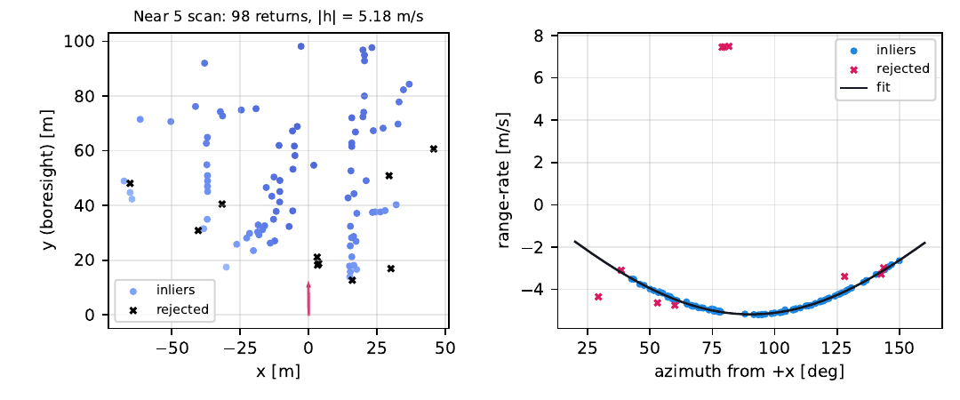
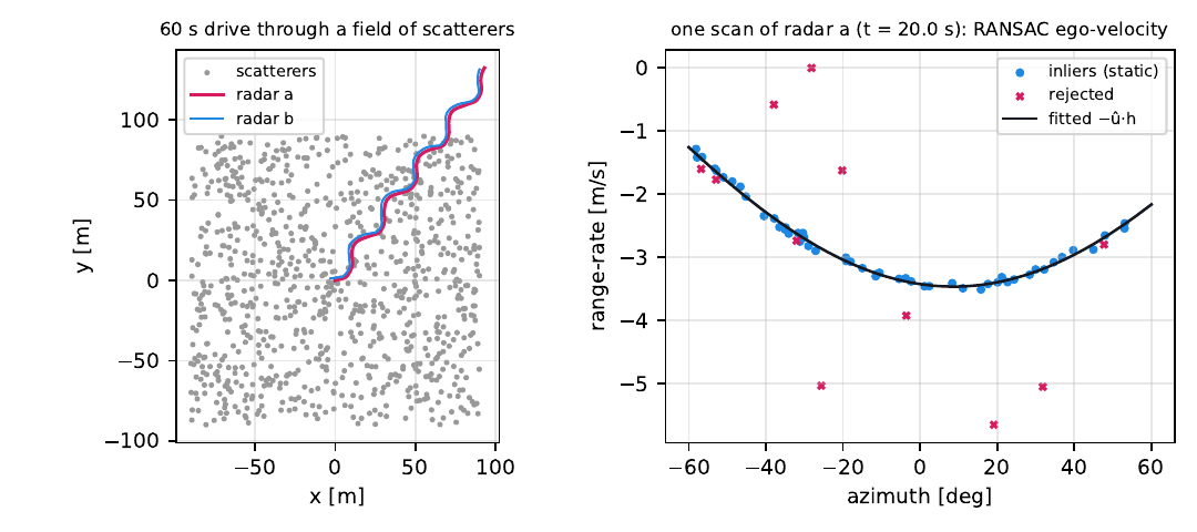
A static target at azimuth θ has range-rate −[cos θ, sin θ]·h. Fifty-odd returns per scan, a two-point RANSAC to drop moving cars and multipath, then linear least squares with a covariance. One velocity vector per radar per scan.

The estimated frame of radar b snapping into place as the batch solver converges

2 · Fuse

One batch problem

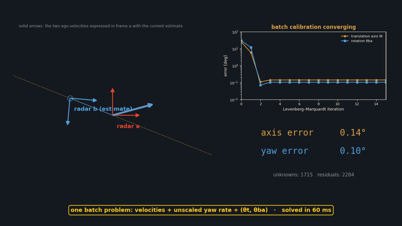
h_b = R(θ_ba)(ω_γ u_⊥ + v_a). Only the yaw and the translation axis are identifiable, since a yaw rate and a baseline scale trade off. Levenberg–Marquardt over every velocity and yaw rate plus the two angles, from a closed-form start.

Ego-velocity of four radars against the odometry speed of the Endeavour bus

3 · Verify

A shuttle bus with five radars

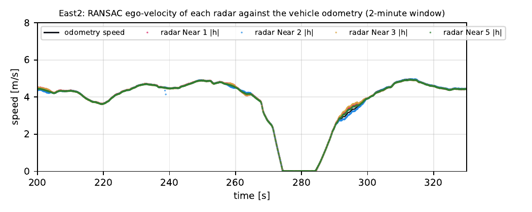
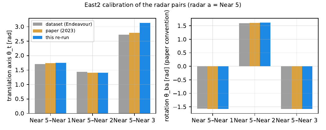
The Endeavour dataset: five Continental ARS430 radars around a bus, six runs of 4–12 minutes. Calibrate on East 2, check on the other five runs. Two of the three available pairs land within 0.01 rad of the paper; the third is weakly identifiable, and says so.

Watch it work

Four short loops from the re-implementation: what the radars see, how one scan becomes a velocity, how the batch solver snaps the second radar into place, and what happens when the motion is degenerate.

1 · Measure

Two radars, one drive

A simulated vehicle through a field of scatterers: returns coloured by range-rate, × for the moving targets RANSAC rejects, arrows for each radar’s own ego-velocity. Neither radar sees the other.

2 · RANSAC

One scan → one velocity

A static return’s range-rate is −[cos θ, sin θ]·h. Two-point hypotheses flash until a consensus set appears; the inliers give h by least squares, with a covariance.

3 · Fuse

The batch problem converging

From a start 25° / 30° away, Levenberg–Marquardt with the Schur complement over every time step lands within 0.1° in four iterations; 1,715 unknowns, 60 ms.

4 · Identifiability

When it cannot work

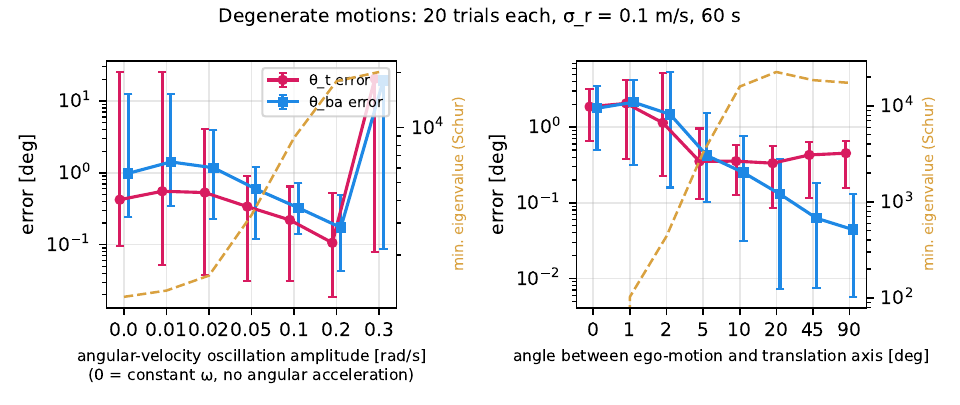
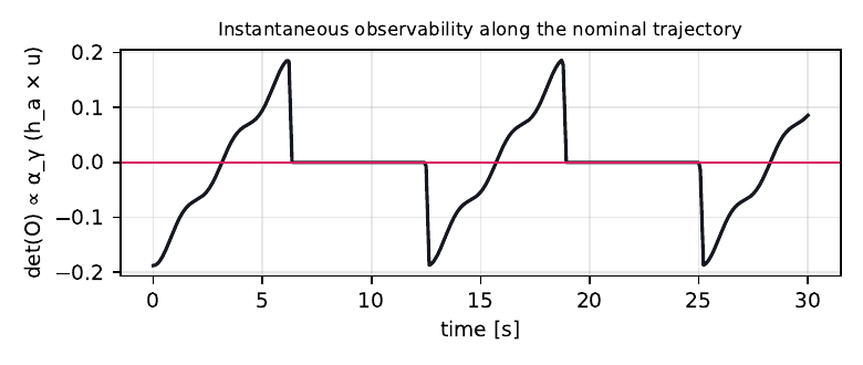
Drive straight along the baseline axis and the information about the axis vanishes exactly, as det O ∝ α (h_a × u) predicts; five degrees of yaw are enough to bring it back.

Try it live

LIVE DEMO · runs in your browser

Place radar b, drive, calibrate

Drag radar b anywhere on the vehicle (or use the sliders), pick the noise, the run length and the kind of motion, then press Drive & calibrate. The drive is simulated at 14 Hz, both ego-velocity streams are generated with the noise you chose, and the paper's solver runs iteration by iteration: closed-form initialisation, then Levenberg–Marquardt with the Schur complement over every time step. The log is the solver's own output.

baseline axis θt yaw θba baseline length ego-velocity noise σ run length motion perturb the initial guess

no run yet

solver log will appear here

Method

A radar cannot see its own rotation, but it can see its own velocity: every static scatterer returns a range-rate equal to minus the projection of the ego-velocity on its line of sight. Two radars rigidly mounted on a body see two velocities of the same body at two different points, and the difference between them is the lever-arm term ω × t. In the plane that term always points along the perpendicular of the translation, so the batch model is

ha = va + na, hb = R(θba) ( ωγ u⊥ + va ) + nb, u = [cos θt, sin θt]

with ω_γ = ω |t| the unscaled yaw rate. Scaling the yaw rate up and the baseline down leaves the data unchanged, so the paper fixes |t| = 1 and estimates the axis θ_t ∈ [0, π) and the yaw θ_ba, which are exactly the two parameters that drift in service and are hardest to measure by hand. The cost is the weighted sum of both residuals over every time step (paper eq. 12).

Front end: RANSAC least squares per scan, 200 hypotheses at once, covariance from the residuals.
Initialisation: yaw from the velocity pairs of equal magnitude, axis from the residual b = Rᵀh_b − h_a ≈ ω_γu_⊥, then a linear solve for the states.
Solver: analytic Jacobians, Schur complement over the 3×3 per-time blocks, so a 2-minute run costs 60 ms; the covariance of (θ_t, θ_ba) and its smallest eigenvalue come for free.
Identifiability: det O ∝ α_γ (h_a × u): the yaw rate must change, the body must move, and not along the translation axis. Checked numerically below.

numpy + scipy onlyno ROS (pure-Python bag reader)fixed seeds16 unit tests

Scatterer simulation: trajectories of both radars and one scan with the RANSAC fit — **Scatterer-level pipeline.** Sixty seconds through 900 random scatterers with 12 % moving targets, both radars scanning at 14 Hz. The RANSAC fit recovers each ego-velocity to 2 cm/s median; the calibration from the valid pairs lands at 158.06° / 95.11° against 158.20° / 95.00°.

Nominal simulation trajectory: ego-velocity and yaw rate — **The paper's nominal trajectory** (its Fig. 2), taken from the archived MATLAB generator: a periodic velocity and a yaw rate that is zero half of the time, which is exactly where det O vanishes.

Simulation studies

Setup

The setup: what is given, what is estimated

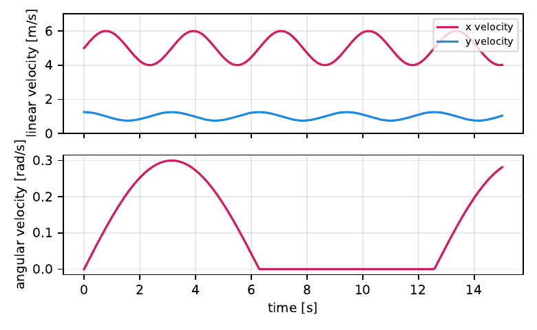
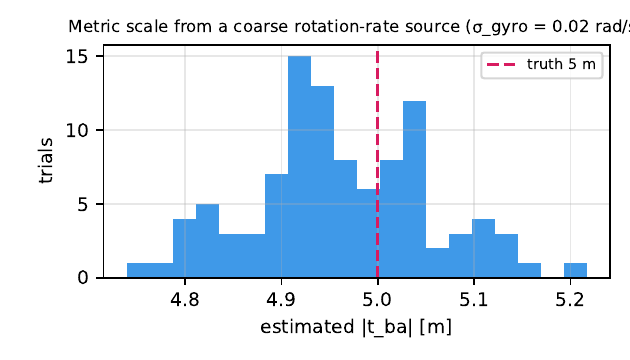
The paper’s nominal drive (its Fig. 2) with the noise being added to both velocity streams, and the ledger of knowns, unknowns and ground truth used for every trial.

Recording

The campaign, recorded

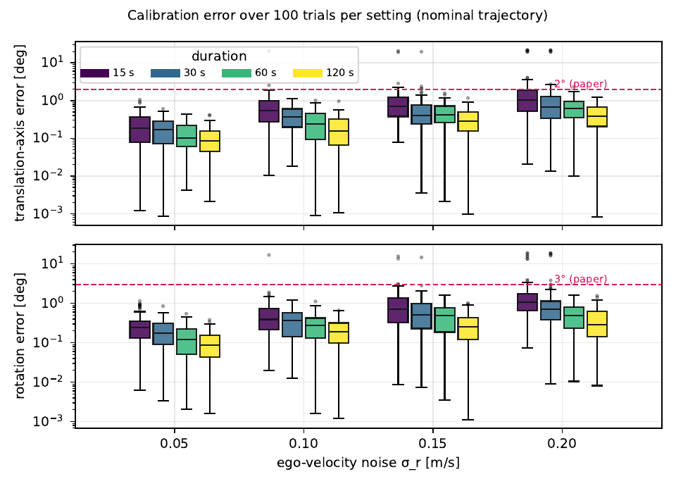
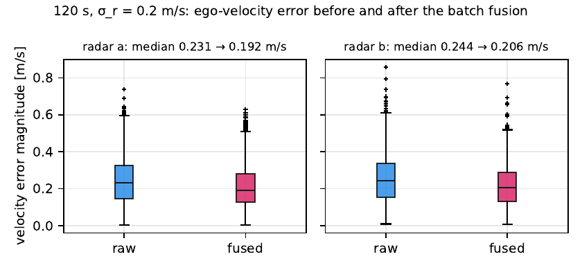
Sixteen noise / duration settings, one hundred seeded trials each. Every dot is one 60-ms solve landing on the error plot; the histograms fill as the campaign runs. Four settings are shown.

Given

Two ego-velocity streams at 14 Hz with isotropic noise σ_r ∈ {0.05, 0.10, 0.15, 0.20} m/s.
Run lengths 15, 30, 60 and 120 s.
Nothing else: no odometry, no IMU, no map.

Estimated

θ_t and θ_ba.
The velocity of radar a and the unscaled yaw rate ω_γ at every step (3M states).

Ground truth

θ_ba = 90°, baseline 5 m along the x axis of radar a (θ_t = 0).
Yaw rate max(0.3 sin(t/2), 0): zero half of the time, so det O vanishes periodically.
100 seeded trials per setting: 1,600 solves in 141 s.

Box plots of axis and rotation errors per noise level and duration — **Paper Fig. 3, re-run.** Absolute error of the translation axis (top) and the rotation (bottom) over 100 trials for each noise level (x axis) and duration (colour). Dashed: the paper’s 2° / 3° envelope. Every trial longer than 30 s at σ ≤ 0.15 m/s sits inside it; the isolated 20° points are wrong local minima reached from a poor closed-form start on the shortest, noisiest runs.

Raw versus fused ego-velocity error for both radars — **Paper Fig. 4.** Because the batch problem ties both radars to one motion, the fused velocities beat the raw ones: median error 0.231 → 0.192 m/s (a) and 0.244 → 0.206 m/s (b) at σ = 0.2 m/s; 3.6 ± 0.3 cm/s averaged over 100 trials, the paper says 4.

σ_r [m/s]	T [s]	θ_t median [°]	θ_t p95	θ_t max	θ_ba median [°]	θ_ba p95	θ_ba max	reported 1σ θ_t / θ_ba	inside 2° / 3°
0.05	15	0.19	0.61	1.1	0.24	0.88	1.2	0.36 / 0.36	100 %
0.05	120	0.08	0.27	0.4	0.09	0.26	0.4	0.13 / 0.12	100 %
0.10	15	0.54	1.67	20.6	0.39	1.49	16.8	0.71 / 0.72	98 %
0.10	60	0.24	0.82	1.0	0.27	0.74	1.1	0.36 / 0.35	100 %
0.10	120	0.16	0.45	1.0	0.19	0.61	0.7	0.26 / 0.25	100 %
0.15	30	0.40	1.59	19.8	0.51	1.72	14.7	0.71 / 0.78	96 %
0.15	120	0.29	0.77	1.2	0.26	0.87	1.0	0.38 / 0.37	100 %
0.20	15	1.05	19.5	21.8	1.08	13.4	18.9	1.36 / 1.48	76 %
0.20	60	0.63	1.50	2.4	0.50	1.28	1.6	0.70 / 0.68	99 %
0.20	120	0.38	1.02	1.2	0.28	1.07	1.6	0.49 / 0.49	100 %

← scroll the table sideways →

Ten of the sixteen settings; all are in the report. The reported 1σ tracks the empirical spread.

Degeneracy sweeps: constant yaw rate and ego-motion aligned with the translation axis — **The two degenerate motions, measured.** Left: the yaw-rate oscillation is shrunk to zero (constant ω): the errors grow 4–6× and the information eigenvalue (gold) drops 15×, but the problem stays solvable because the heading still changes. Right: driving along the translation axis. At 0° the smallest eigenvalue is numerically zero, the unobservable case the paper’s determinant predicts; 5° away it is back to nominal.

Observability determinant along the nominal trajectory — **det O along the nominal trajectory:** zero whenever the yaw rate is constant, which the paper’s own trajectory does for half of every period.

Histogram of the recovered translation magnitude with a coarse gyro — **Paper Table IV.** Add any coarse yaw-rate source (here 0.02 rad/s noise) and the unscaled yaw rate gives the metric baseline: 4.96 ± 0.09 m for a 5 m truth.

Endeavour dataset

Forty seconds of the real East 2 run: the four available Continental ARS430 radars around the shuttle bus, their returns coloured by range-rate in the vehicle frame, the RANSAC inliers, each radar’s ego-velocity arrow, the speeds against the odometry, and the lever-arm signal (the speed difference between a side radar and the front radar) that carries the calibration information.

The Xi’an Jiaotong “Endeavour” shuttle bus carries five ARS430 radars (front, and two on each side) sampled at 13 Hz, plus an RTK-corrected odometry. Six loops of 4–12 minutes. The archived raw bags were converted to point clouds twice, and the two conversions do not agree: in the July-2022 set the azimuth is mirrored and offset by 3.3°, and the ego-velocities computed from it over-read the odometry speed by 7 % on the side radars but only 2.6 % on the front one. With such a between-radar bias the batch problem prefers a degenerate answer. The September-2022 set has consistent azimuths, speed ratios of 0.995–0.999 on every radar, and is what everything here uses. It lacks radar Near 4, so three of the paper’s four pairs could be re-run.

Pipeline: returns beyond 1 m with |ṙ| < 10 m/s → RANSAC at 0.1 m/s (the paper’s 0.025 m/s only passes 5–30 % of these scans; the ARS430 spread is 0.05-class) → interpolate radar b onto radar a’s clock → drop pairs slower than 0.05 m/s → batch calibration with per-scan covariances, about 6,470 pairs each.

Ego-velocity magnitudes of the four radars against the odometry speed — **Front end on real data.** RANSAC ego-velocity magnitudes of the four radars against the odometry speed over a two-minute window of East 2; 99.8 % of the scans yield an estimate.

One real radar scan: returns and the fitted ego-velocity — **One real scan** of the front radar: inliers, rejected returns and the fitted range-rate curve.

pair (a = Near 5)	pairs M	dataset θ_t	dataset θ_ba	paper θ_t	paper θ_ba	re-run θ_t	re-run θ_ba	1σ θ_t / θ_ba [°]	Δ to dataset [°]
Near 1 (rear, 5.7 m)	6477	1.71	−1.57	1.74	−1.58	1.754	−1.583	0.05 / 0.02	+2.5 / +0.8
Near 2 (rear, 5.8 m)	6472	1.44	1.59	1.41	1.61	1.409	1.615	0.05 / 0.02	−1.9 / −1.6
Near 3 (front side, 0.8 m)	6478	2.73	−1.58	2.79	−1.58	3.134	−1.573	0.06 / 0.003	+23.2 / −0.1

← scroll the table sideways →

Radians, in the paper’s convention (its rotation matrix is the transpose of the one used here, so the sign of θ_ba is flipped in the code). East 2 is the calibration run.

Bar chart of the calibration parameters: dataset, paper, re-run — **Paper Table I.** For the two long-baseline pairs the re-run reproduces the 2023 estimates to 0.015 rad and the dataset’s extrinsics to 2.5°. Near 5–Near 3 has a 0.83 m baseline, so its lever-arm signal is at most 0.25 m/s, comparable to the noise: the axis comes out 23° off and the reported 1σ is over-confident there.

Held-out velocity errors per run for dataset, paper and re-run parameters — **Paper Table III.** Mean velocity-error magnitude on the five other runs with each parameter set (yaw rate chosen per time step, unit moment arm). The re-run wins on every run for the two long-baseline pairs (9–18 mm/s against 17–28 mm/s with the dataset values); for the weak pair the dataset’s axis is better on four of five runs, which is the honest way to read the 23°.

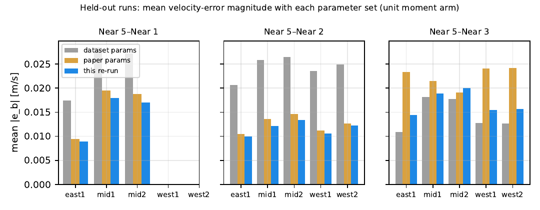
run	Near 5–Near 1 [m/s]			Near 5–Near 2 [m/s]			Near 5–Near 3 [m/s]
run	dataset	paper	re-run	dataset	paper	re-run	dataset	paper	re-run
east1	0.0174	0.0095	0.0089	0.0207	0.0105	0.0099	0.0109	0.0233	0.0145
mid1	0.0284	0.0195	0.0179	0.0258	0.0136	0.0121	0.0182	0.0215	0.0189
mid2	0.0272	0.0188	0.0170	0.0264	0.0146	0.0133	0.0178	0.0191	0.0200
west1	—	—	—	0.0236	0.0112	0.0106	0.0127	0.0240	0.0154
west2	—	—	—	0.0248	0.0127	0.0122	0.0126	0.0242	0.0157

← scroll the table sideways →

What the re-run found

Three things that are not in the paper and that anyone re-using the method or the dataset should know.

1

A mirrored bag makes the batch problem lie

The per-time yaw rate ω_γ^j is a free variable, so the model can absorb any residual along the perpendicular of the translation axis. If the two radars' speeds disagree by a few percent, the cheapest explanation is a wrong yaw plus an axis chosen so that its perpendicular soaks up the difference: on the mirrored July-2022 bags every pair converged to θ_t ≈ 93° with the yaw 25–30° off, at a lower cost than the truth. The cure was the data, not the solver; the diagnostic is the odometry speed ratio, which should be 1.00 on every radar.

2

Short baselines are weakly identifiable

The information about the axis scales with |ω| |t|. For the two rear radars that signal is up to 1.7 m/s; for the front-side pair it is 0.25 m/s at most, the same size as the ego-velocity noise. The solver still converges from both the automatic and the dataset-based start to one crisp answer with a 0.06° reported sigma, and that answer is 23° from the dataset's. The covariance is exact for the model; the model is not the whole story when the excitation is that small. A prior on the axis, or a longer run with more turning, is the fix.

3

The basin of attraction is about 25° wide

Starting the batch solver 38° / 45° away from the truth lands in a spurious minimum 63° / 60° away with 30× the cost; starting 25° / 30° away converges in four iterations. The closed-form initialisation is inside that basin in every 60-s run and in 76–98 % of the 15-s runs at the highest noise, which is where the 20° outliers of the simulation sweep come from. Whenever the yaw rate changes sign with a small amplitude the initialiser also fails, while the batch problem itself is fine from a better start.

Full demo

63 s: the scatterer simulation with both radars' returns and ego-velocity streams, the batch problem converging from a deliberately wrong start, the simulation sweep and the degeneracy check, the Endeavour ego-velocities against odometry with the calibration read-out, and the held-out evaluation.

Reproduce

The re-implementation is an installable package, r2rcal, with a pytest suite and a harness that regenerates every figure, table, the report and both videos from scratch (numpy, scipy, matplotlib, the pure-Python rosbags reader; ffmpeg for the videos). The Endeavour bags are not redistributed; the report says which conversion to use.

pip install -e . && pytest # 16 tests cd experiments python sim_sweep.py # 1600 solves, ~2.5 min python sim_pipeline.py # scatterers → RANSAC → calibration ENDEAVOUR_DIR=/bags python run_endeavour.py # 6 runs, stage 1 + 2 python fig_endeavour.py && python make_tables.py && (cd ../docs && make) python make_video.py # thumbnail + full demo

radar-radar-calibration on GitHub Technical report Paper

Credits

Paper. Qilong Cheng, Emmett Wise (equal contribution) and Jonathan Kelly, Space & Terrestrial Autonomous Robotic Systems Laboratory, University of Toronto Institute for Aerospace Studies. IEEE/ASME AIM 2023.

Data. Endeavour Radar Dataset, Institute of Artificial Intelligence and Robotics, Xi'an Jiaotong University (five ARS430 radars, RTK/INS odometry).

2026 re-run. Python re-implementation, simulation and scatterer studies, the Endeavour re-run from the raw bags, the report, the videos and this page. The original MATLAB solver and ego-velocity tools were consulted for the trajectory generator and the dataset conventions.