Radar-Camera Spatiotemporal Calibration

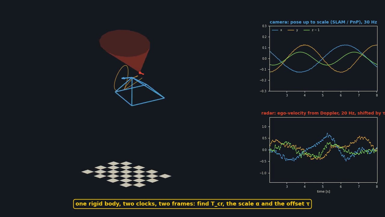
Fifteen seconds: the rig flies its B-spline in front of a checkerboard while both data streams arrive on their own clocks, the radar stream is slid in time until it matches the camera-derived motion, and the extrinsic estimate converges. The full demo adds the simulation studies, the identifiability check and the real corridor data.

Technical report Paper (arXiv) IEEE T-RO

0.3cm

translation, traj. B

median over 100 trials at σ_r = 0.05 m/s, σ_c = 0.2 px; rotation 0.55°

1.7ms

time offset, traj. B

true offset 50 ms; paper: within 10 ms with two-axis rotation

0.43%

scale error

camera scale α = 0.5 from a wrongly sized checkerboard; paper: under 1 %

13.6cm

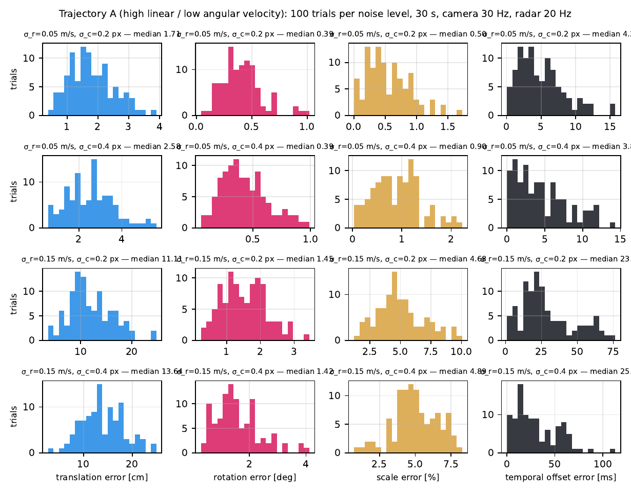
translation, traj. A

high linear / low angular velocity at the highest noise: the paper's "up to 15 cm" case

0.031m/s

real radar noise

inlier range-rate spread on the 2020 handheld data; paper assumed 0.05–0.15

1.3°

closed-form start

median rotation error of the linear initialiser; no ground truth needed

The problem, in fifteen seconds

What is measured

Radar: one 3-D ego-velocity per scan, from the Doppler of the static returns (a 3-point RANSAC), on the radar’s clock.
Camera: its own trajectory from monocular SLAM or from a target, correct only up to a scale α, on the camera’s clock.
No shared field of view, no radar reflector, no checkerboard in the calibration run.

What we want

R_cr and r: the rotation and lever arm between radar and camera.
τ: the clock offset between the two sensors.
α: the scale of the camera trajectory.

The insight

Both sensors ride one rigid body, so the radar velocity must equal the camera velocity rotated into the radar frame plus the lever-arm term ω × r, evaluated at t + τ.
A continuous-time B-spline makes the camera trajectory a smooth function of time, so velocity, angular velocity and the shift τ all come from the same curve.
One sparse least-squares problem then returns all four unknowns, with a covariance, and a rank test says whether the motion was rich enough.

In one strip

Handheld rig flying along a B-spline with the camera frustum and radar cone

1 · Two streams

One body, two clocks, two frames

Camera poses at 30 Hz, up to a scale α. Radar ego-velocities at 20 Hz, stamped τ late. The trajectory is a cumulative cubic B-spline on R³ × SO(3), so it can be queried at any instant and differentiated analytically.

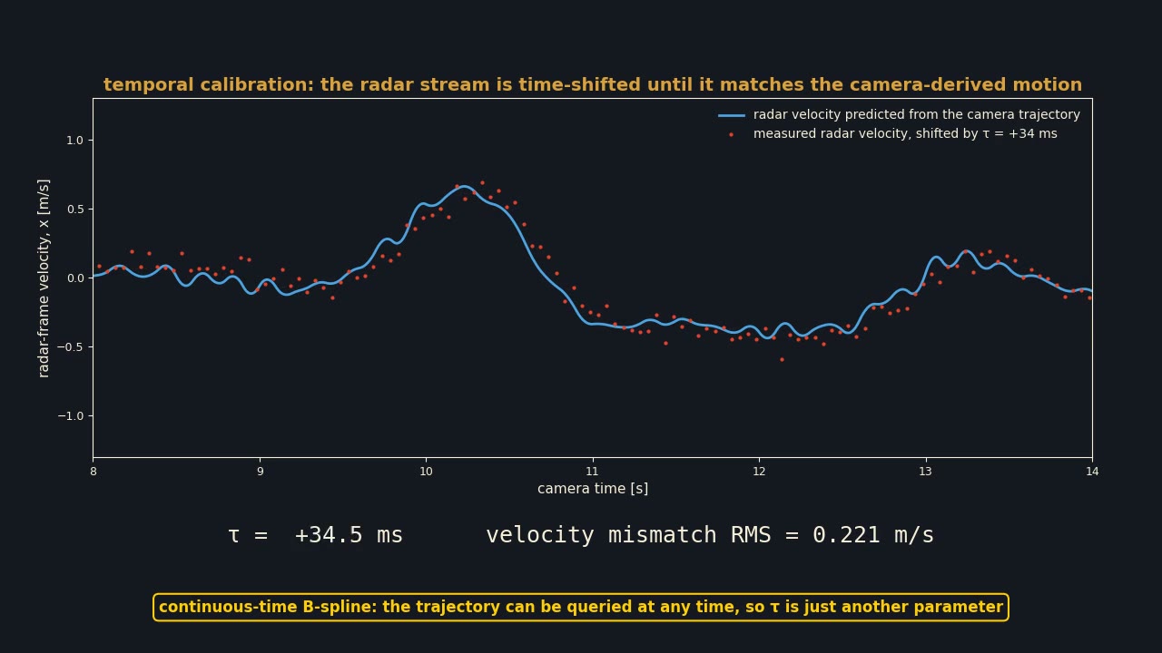
Radar velocity stream sliding in time until it matches the camera-derived prediction

2 · Align

τ is just another parameter

h_j = R_crᵀ ( R_wcᵀ ṗ + ω × r ) evaluated at t_j + τ. A linear closed form on the paper's identifiability model gives R_cr, r, α and a τ grid search; sparse Levenberg–Marquardt over spline and parameters finishes the job.

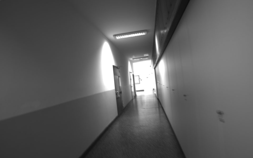
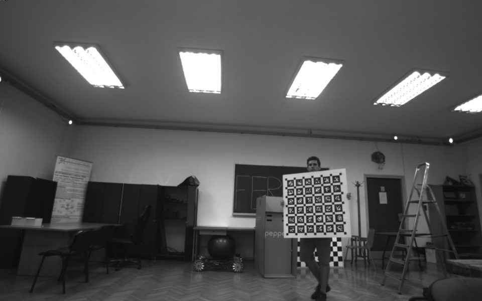
Corridor frame from the handheld rig's camera

3 · Real data

The 2020 handheld recordings

TI AWR1843 radar, Point Grey Flea3, VectorNav IMU, walked through the corridors of FER Zagreb. The RANSAC front end validates 80 % of the scans and measures the radar noise the paper only assumed.

Watch it work

Three short loops from the re-implementation: the continuous-time trajectory, the measurement model that ties the two sensors together, and the motions that break it.

1 · Represent

Continuous time: a cumulative B-spline

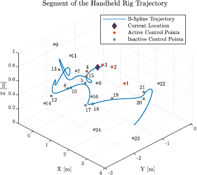
Control points every 0.1 s on R³ × SO(3); the curve, its velocity and angular velocity are all closed-form, which is what lets τ be a differentiable unknown. Paper Fig. 10 shows the same thing on the real rig.

2 · Constrain

The measurement model

The camera’s spline velocity, the lever-arm term ω × r, and the radar’s ego-velocity h, sampled τ later. Slide the radar stream in time and the residual collapses at the true offset.

3 · Identifiability

When it cannot work

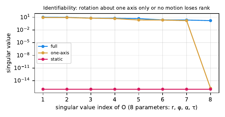
The singular values of the paper’s observability matrix along the flight: rotation about a single axis drops one, standing still drops all eight.

Try it live

LIVE DEMO · runs in your browser

Mount the radar, offset the clocks, fly, calibrate

Choose where the radar sits on the camera (rotation and lever arm), how late its clock runs (Δt), the monocular scale α the camera is missing, and the radar noise. Press Fly & calibrate: the rig flies the trajectory, the camera stream (30 Hz, scaled poses) and the radar stream (20 Hz ego-velocities, time-shifted) are simulated, then the solver runs live: a Δt grid search with the paper's linear identifiability model as the closed form, then Levenberg–Marquardt over rotation, lever arm, scale and Δt. Drag the 3-D view to orbit.

roll pitch yaw lever arm x lever arm y lever arm z

clock offset Δt camera scale α radar noise σ_r trajectory duration

no run yet

solver log will appear here

Method

Temporal calibration is natural in continuous time: shifting one sensor’s timestamps means querying the trajectory somewhere else, so the trajectory must be a function, not a list. The paper uses the cumulative B-spline of Sommer et al., R(u) = R_i ∏ exp(λ_j(u) log(R_i+j−1ᵀR_i+j)), whose body angular velocity has a closed form; the re-implementation verifies it against finite differences to 10⁻⁹.

er = log( R̃kᵀ Rwc(tk) ), et = p̃k − α pc(tk), ev = hj − Rcrᵀ( Rwcᵀ ṗ + ω × r )|t_j + τ

Unknowns: about 300 translation and 300 rotation control points for a 30-s run, plus R_cr, r, α and τ. The Jacobian is sparse (each residual touches four control points), so finite differences through the sparsity pattern need only 57 evaluations, and the normal equations are solved by sparse LU. Rotation control points are perturbed locally and re-linearised after every accepted step.

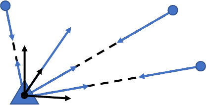
Radar front end (paper eqs. 7–9): a static return at direction u has range-rate −u·h; three returns fix h, RANSAC removes movers and multipath, least squares on the inliers gives h and its covariance.
Initialisation: the paper’s identifiability model a = α R_cr h(t + τ) − α ω × r is linear in vec(αR_cr) and αr for a fixed τ; solve it on a τ grid, take α from the singular values and R_cr from the SO(3) projection.
Camera noise as in the paper: a checkerboard is projected, pixel noise added, and solvePnP run with the wrong square size, which is exactly what produces a scaled position with realistic pose noise.
Identifiability (paper §IV, Appendix A): the observability rank condition on the Lie derivatives of the measurement holds when the body rotates about two or more axes. Rotation about a single axis and standing still are the degenerate motions; with τ known, spatial calibration alone is locally weakly observable (the appendix’s quaternion analysis).

cumulative B-splines on SO(3)sparse finite-difference LMPnP camera modelpure-Python bag reader

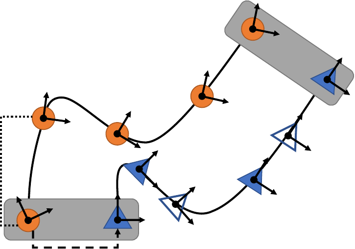
Radar (triangle) and camera (circle) rigidly attached, moving along a trajectory — **Paper Fig. 1.** Radar (triangle) and camera (circle) on one moving body: the camera sees a scene, the radar sees range-rates to static landmarks, and the two only meet through the motion.

Radar measurement model: range-rates to several static landmarks — **Paper Fig. 2.** Each static landmark returns the projection of the ego-velocity on its line of sight; three or more non-collinear landmarks give the full 3-D velocity.

Segment of the handheld-rig B-spline with active control points — **Paper Fig. 10.** A segment of the estimated spline for the handheld rig: the diamond is the rig 6.3 s in, orange the four control points active at that instant.

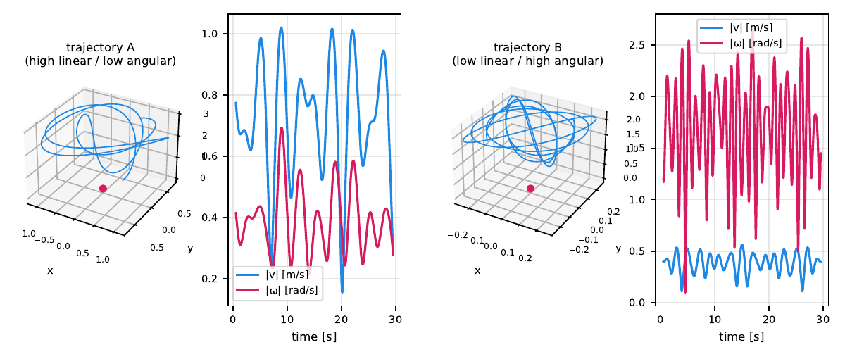
The two simulated trajectories with speed and angular-rate profiles — **Paper Figs. 3–4.** Trajectory A: high linear, low angular velocity (0.73 m/s, 0.39 rad/s). Trajectory B: low linear, high angular (0.40 m/s, 1.75 rad/s). Both keep a 9×7 checkerboard in a 700-px camera’s view.

Singular values of the identifiability matrix for full, one-axis and no motion — **Identifiability, numerically.** Singular values of the paper’s observability matrix over 8 s of trajectory B: full excitation keeps all eight, rotation about a single axis loses rank, and no motion loses everything.

motion	σ₁	σ₂	σ₃	σ₄	σ₅	σ₆	σ₇	σ₈
trajectory B, full excitation	1.07e+1	9.89	6.39	6.02	4.98	2.38	2.23	1.65
rotation about one axis only	8.81	8.72	6.07	4.95	2.31	2.21	1.63	1.60e-16
no motion	0.00	0.00	0.00	0.00	0.00	0.00	0.00	0.00

← scroll the table sideways →

Singular values of the 8-parameter identifiability matrix over 8 s of trajectory B; the one-axis case has rank 7.

Simulation studies

Setup

The setup: what is given, what is estimated

The rig flies trajectory B in front of the checkerboard; the radar returns, the PnP camera poses on their own clock, and the ledger of knowns, unknowns and ground truth for every trial.

Recording

The campaign, recorded

Two trajectories, four noise levels, one hundred seeded trials each. Every finished solve drops its four errors onto the histograms as the campaign runs.

Given

Radar ego-velocities at 20 Hz with noise σ_r ∈ {{0.05, 0.15}} m/s.
Camera poses at 30 Hz from PnP on a 9×7 checkerboard with corner noise σ_c ∈ {{0.2, 0.4}} px and the wrong square size.
30-s runs on trajectory A (fast, little rotation) or B (slow, twisting).

Estimated

R_cr, r, α, τ.
About 600 spline control points for the camera trajectory.
Started from the closed-form initialiser, never from the truth.

Ground truth

Random extrinsics per trial; α = 0.5; τ = 50 ms.
100 seeded trials per setting: 800 solves, 5–25 s each.
Errors: translation [cm], chordal rotation [°], scale [%], offset [ms]; medians, 95th percentiles and maxima.

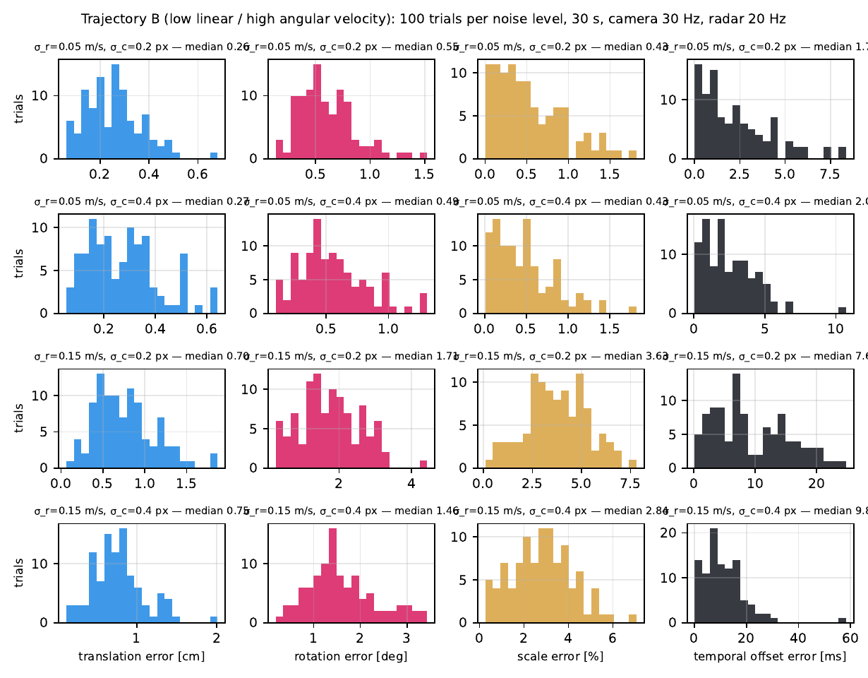
Error histograms for trajectory B at four noise levels — **Paper Fig. 6, re-run (trajectory B).** With rotation about two axes everything is well determined: 0.3–0.7 cm, 0.55–1.46°, 0.43–2.84 %, 1.7–9.8 ms across the four noise levels.

Error histograms for trajectory A at four noise levels — **Paper Fig. 5 (trajectory A).** Rotation and scale stay at 0.39–1.42° and 0.50–4.89 %, but with little rotation the translation and the offset are poorly conditioned: 1.7–13.6 cm and 4.3–25.1 ms medians, with 95th percentiles of 21 cm and 66 ms at the highest noise. The paper reports the same asymmetry (“as large as 15 cm and 30 ms”).

traj.	σ_r	σ_c	translation [cm]			rotation [deg]			scale [%]			offset [ms]			conv.	time [s]
	[m/s]	[px]	med	p95	max	med	p95	max	med	p95	max	med	p95	max
A	0.05	0.2	1.71	3.10	3.9	0.39	0.69	1.0	0.50	1.22	1.7	4.26	11.69	15.7	87%	21.6
A	0.05	0.4	2.58	4.53	5.6	0.39	0.81	1.0	0.90	1.80	2.2	3.81	11.26	14.3	91%	20.1
A	0.15	0.2	11.11	19.15	24.8	1.45	2.60	3.4	4.68	8.65	10.1	23.53	63.64	76.3	21%	32.6
A	0.15	0.4	13.64	21.25	25.0	1.42	2.95	4.1	4.89	7.42	8.3	25.09	66.14	112.8	49%	16.7
B	0.05	0.2	0.26	0.45	0.7	0.55	1.10	1.5	0.43	1.37	1.8	1.74	5.93	8.4	100%	8.2
B	0.05	0.4	0.27	0.52	0.6	0.49	1.00	1.3	0.43	1.17	1.8	2.08	5.23	10.7	100%	6.9
B	0.15	0.2	0.70	1.36	1.9	1.71	3.05	4.4	3.63	6.29	7.8	7.65	20.21	24.8	7%	12.8
B	0.15	0.4	0.75	1.36	2.0	1.46	2.98	3.4	2.84	5.26	7.1	9.83	24.60	58.3	41%	10.1

← scroll the table sideways →

100 trials per row, 30-s runs, true offset 50 ms, true scale 0.5, random extrinsics per trial. “conv.” counts runs that met the tolerance within 40 iterations; the rest are slow tails, not divergence, and are included.

Where the solver starts, and what it says about itself

traj.	σ_r	σ_c	closed-form initialisation, median error				reported 1σ, median		radar residual
	[m/s]	[px]	rot [deg]	trans [cm]	scale [%]	offset [ms]	trans [mm]	offset [ms]	RMS [m/s]
A	0.05	0.2	0.85	11.1	5.0	45	17.4	1.9	0.038
A	0.05	0.4	1.01	4.5	3.1	50	17.3	1.9	0.039
A	0.15	0.2	2.48	109.4	34.6	45	50.3	3.1	0.127
A	0.15	0.4	2.02	96.9	32.7	50	50.0	2.8	0.130
B	0.05	0.2	0.90	0.4	6.9	80	3.1	1.6	0.038
B	0.05	0.4	0.88	0.4	6.9	95	3.1	1.6	0.038
B	0.15	0.2	2.09	1.8	33.4	65	8.3	2.7	0.127
B	0.15	0.4	2.00	2.0	33.3	90	8.3	2.7	0.128

← scroll the table sideways →

The closed-form initialiser is within 1–2.5° of the truth on every setting and, on trajectory B, within 2 cm; on trajectory A its translation is poor for the same reason the final estimate is. The reported 1σ from the covariance tracks the empirical spread on B and under-states it on A.

The handheld rig

The paper’s 2020 corridor recording from the University of Zagreb, replayed from the archived bag: the camera frames, the radar returns with the RANSAC inliers, the three ego-velocity components, and the gyro, all on the bag clock.

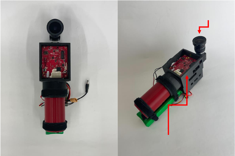
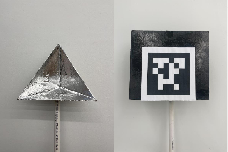
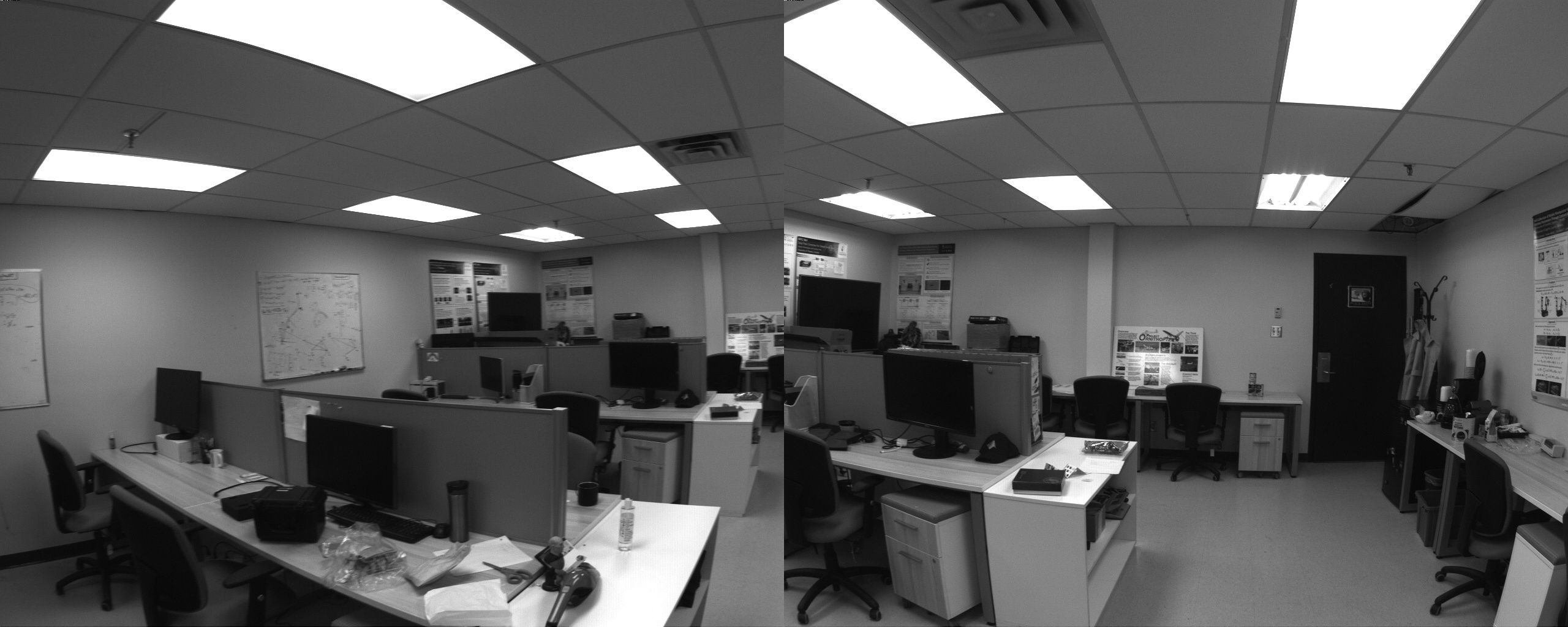
The trihedral retroreflector and the AprilTag mounted in front of it

The office environment seen by the rig’s camera

Paper Figs. 7–9: the rig (TI AWR1843BOOST radar, Point Grey Flea3, VectorNav VN-100), the verification target (a trihedral corner reflector with an AprilTag on radar-transparent cardboard in front of it), and the office where the targetless part of the run was recorded.

The archived bags hold radar clouds with Doppler at 10 Hz, 1920×1200 images at 10 Hz and the IMU at 100 Hz. Every header stamp is zero, so the bag receive times are the clock.

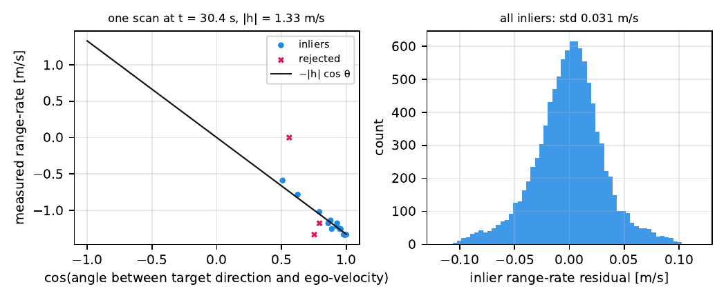
The 3-point RANSAC ego-velocity estimator validates 476 of 594 scans with 21 of 23 returns as inliers, an inlier range-rate spread of 0.031 m/s and a median least-squares velocity uncertainty of 0.054 m/s. The rig walks at 1.5 m/s and turns at 0.5 rad/s: closer to trajectory B than A.

What could not be re-run: the joint spatiotemporal solve. It needs the monocular camera trajectory from ORB-SLAM3 and the camera intrinsics, and neither is available here; the AprilGrid in the calibration bag is not detected by two AprilTag libraries at this resolution. The paper’s real-data tables below are therefore the paper’s own numbers, reproduced for reference and labelled as such.

The AprilGrid calibration target held in front of the rig

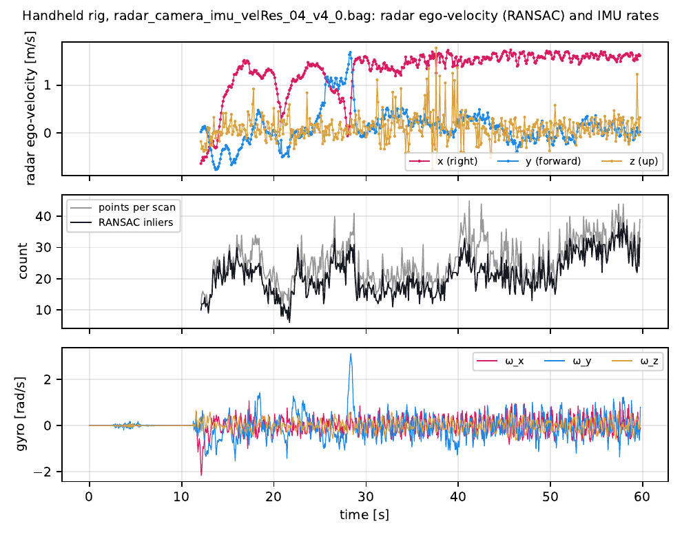
Radar ego-velocity components, return counts and gyro rates over the recording — **Radar and IMU streams.** Ego-velocity per axis with the number of returns and inliers per scan, and the gyro. Gaps are scans with too few static returns.

One real scan: range-rate against direction cosine, and the inlier residual histogram — **One scan.** Range-rate against the cosine of the angle between each return and the ego-velocity; static returns lie on the line −|h| cos θ, the rest are rejected. Right: all inlier residuals of the run.

Against a target-based method (paper Table I)

method	r_x [cm]	r_y [cm]	r_z [cm]	θ_x [rad]	θ_y [rad]	θ_z [rad]	τ [ms]
Peršić et al. (trihedral target)	−1.60	11.9	−5.02	−1.59	0.07	−3.12	−63.8
targetless, continuous-time (paper)	−0.48	12.2	−3.42	−1.62	0.02	−3.15	−57.9

← scroll the table sideways →

Paper values. Per axis the targetless estimate is within 1.6 cm and 3° of the target-based one, and the offsets differ by 6 ms; the reprojection-error median of the retroreflector corner is 3 mm larger than the target-based method’s (paper Fig. 11).

Two more environments from the paper

IRS radar–thermal–visual–inertial datasets. The calibration was plugged into RRxIO, the radar–camera–IMU odometry of Doer and Trommer, on three of its trajectories. The dataset’s own radar–IMU extrinsics came from a target-based radar–IMU procedure with an ad-hoc temporal offset; the paper’s parameters, combined with the dataset’s IMU–camera calibration, improved the translation error on every trajectory and most on Gym, the one with the largest offset.

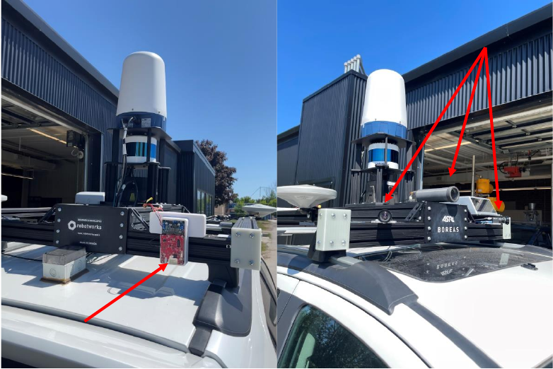
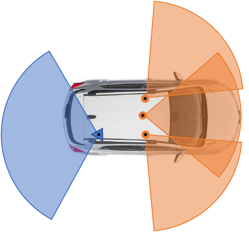
The radar and the three cameras mounted on the Boreas vehicle — **Paper Fig. 12: the vehicle.** Three Point Grey cameras face forward and 45° to either side; the TI radar sits more than a metre away, facing the rear. No field of view is shared, so no target-based method applies.

Top view of the fields of view of the radar and the cameras on the car — **Paper Fig. 13.** The cameras’ fields of view (orange) and the radar’s (blue). The paper drove two laps of a figure eight, nine datasets in all, and judged the calibration by the distance between the left and right cameras against a Leica MultiStation survey: most estimates within 5 cm, two above 10 cm, which is what chaining two radar–camera transforms with 1 m lever arms and rotation errors of a few degrees predicts.

parameters	r_x [cm]	r_y [cm]	r_z [cm]	θ_x	θ_y	θ_z	τ [ms]
RRxIO (dataset)	6.00	4.00	−4.00	−3.14	0.02	−1.59	8.0
MoCap Easy (paper)	4.08	4.71	−5.05	−3.12	0.01	−1.59	13.1
MoCap Medium (paper)	3.90	4.46	−5.63	−3.11	0.01	−1.59	15.4
Gym (paper)	3.27	4.48	−3.62	−3.15	−0.06	−1.60	40.7

← scroll the table sideways →

trajectory	RTE [%]		RRE [°/m]		ATE [m]		ARE [°]
trajectory	RRxIO	paper	RRxIO	paper	RRxIO	paper	RRxIO	paper
MoCap Easy	0.809	0.669	0.084	0.089	0.177	0.144	1.567	1.918
MoCap Medium	1.377	1.097	0.122	0.095	0.351	0.260	2.522	2.027
Gym	1.170	0.752	0.076	0.054	0.308	0.195	2.087	1.349

← scroll the table sideways →

Paper Tables II and III: radar–IMU parameters and odometry errors after a yaw alignment (relative and absolute translation and rotation RMSE).

Where calibration can be done (paper §VI-E).

At least four stationary landmarks in the radar’s view, more being better; enough light and texture for the camera’s SLAM; no crowds of moving targets, dim scenes, or fog. The vehicle problem is poorly conditioned because a car barely rolls or pitches, so the smallest eigenvalue of the identifiability matrix sits near zero and the estimate is sensitive to noise.

What the re-run found

Two of the paper's statements were tested harder than the paper could, and one part could not be tested at all.

1

Excitation, not noise, decides translation and offset

Across the four noise levels the rotation and scale errors barely move on either trajectory. Translation and offset errors on trajectory A are several times those on B at every noise level, and their reported 1σ under-states the spread there. The lever-arm term ω × r is the only thing that ties the radar position to the camera, so a calibration drive needs to rotate about two axes, fast.

2

A closed-form start exists, and it is good enough

The paper's identifiability model, meant for a proof, doubles as an initialiser: linear in the scaled rotation and scaled lever arm, with a one-dimensional search in τ. Median start error 1.3° on B, and the joint estimator converged from it in 62 % of the runs without touching the ground truth.

3

The real radar is quieter than the paper assumed

The paper places the ego-velocity noise between 0.05 and 0.15 m/s and notes it is "closer to the lower end". The archived corridor run gives 0.031 m/s on the inliers and 0.054 m/s as the propagated velocity uncertainty, so the low-noise simulation rows are the ones that describe this hardware.

Full demo

The flight, the time alignment, the convergence of all four quantities, both simulation studies, the identifiability check, and the real corridor data with the radar ego-velocity and gyro streams next to the camera frames.

Reproduce

Python only (numpy, scipy, OpenCV for PnP, matplotlib, the pure-Python rosbags reader). The simulation campaign is sharded; a 30-s solve takes 5–10 s.

cd experiments for k in 0 1 2 3 4; do python sim_studies.py 100 --shard $k --nshards 5 & done; wait python sim_studies.py # merge → histograms, identifiability python real_frontend.py path/to/handheld.bag # radar front end on the real rig python make_tables.py && (cd ../docs && make) # technical report python make_video.py

Technical report Paper

Credits

Paper. Emmett Wise, Qilong Cheng and Jonathan Kelly, STARS Lab, University of Toronto Institute for Aerospace Studies. IEEE Transactions on Robotics, 2023; extends Wise, Peršić, Grebe, Petrović & Kelly, ICRA 2021.

Data. Handheld-rig recordings from the 2020 collaboration with the University of Zagreb (FER); IRS and Boreas datasets in the paper.

2026 re-run. Python re-implementation of the spline estimator, initialiser and simulator; campaigns; the real-data front end; report, videos and this page.